


Table of Contents |
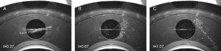
IV. RESULTSA. The Rising Pulsed Jet
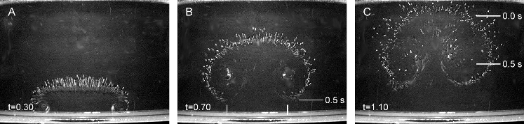
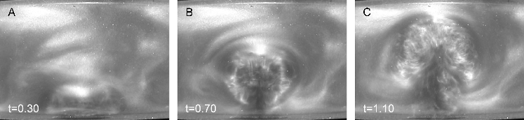
Figures 3 and 4 show the development of the pulsed
jets in a static fluid. Since the jet pulse is relatively short in
time, this produces a single large-scale vortex ring (as in
Sánchez et al.7). The outermost radius of the vortex
ring diverges similarly to the outline of a standard point-source
entrainment plume (Morton et al.15). In Fig. 3 the relatively
smooth laminar flow at the head of this vortex ring is evident in the
trajectory of the bubble tracers released ahead of it. Figure 4 shows
the same pulsed jet rising at the same times as Fig. 3, but in
guanidine. In contrast to Fig. 3, Fig. 4 shows the internal turbulent
behavior. The animated .gif file (ANIMATE
Figure 3:
Figure 3 shows the side view showing the laminar flow
ahead of the pulsed jet in an Ω = 0 static fluid field with a
hydrogen electrolysis pulse of 0.1 s duration
(ANIMATE
Figure 4:
Figure 4 shows the side view of a rising pulsed jet
showing turbulent entrainment in an Ω = 0 static fluid field
with guanidine (ANIMATE
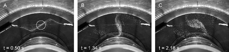
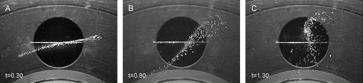
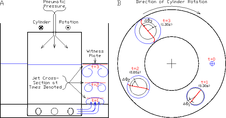
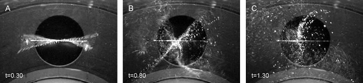
B. The Rotating Pulsed JetFigures 5 and 6 show the rotation of the laminar fluid ahead of the pulsed jet produced from the small and large ports respectively in Ω = const rotation. Figure 7 shows a schematic of the rotation measurements. The vertical position, Fig. 3, and change in angle of the line of bubble tracers of Fig. 6 is shown schematically in Fig. 7. Since the camera rotates with the frame, the top view, Fig. 7(B), shows the angle of rotation with the times and pulsed jet size of Fig. 6.
Figure 5:
Figure 5 shows the top view exhibiting pulsed jet rotation
in an Ω = const fluid flow field with 3.3 cm port (ANIMATE
Figure 6:
Figure 6 shows the top view exhibiting pulsed jet rotation
in an Ω = const fluid flow field with 4.8 cm port (ANIMATE
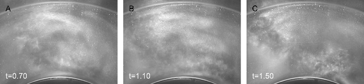
Figure 7: Figure 7 shows the schematic side and top views of the pulsed jet divergence and rotation in an Ω = const rotating frame. A jet is injected into the rotating annulus of water from the port by a pulse of air above the water surface interior to the inner cylinder. As the pulsed jet rises, it expands and rotates relative to the surrounding fluid. The parenthetical times denoted in the top view coincide with the times and views shown in the images in Fig. 6. Figure 8 shows the rotation of the large port pulsed jet when striking the witness plate as observed with guanidine. The further differential rotation of the turbulent flow at the witness plate following the non-turbulent flow at the head of the jet is moderately discernible. Analysis of the original 30 Hz image series of this pulsed jet recording gave the clear impression of further differential rotation of the turbulent flow at the witness plate.
Figure 8:
Figure 8 shows the rotation of the large port pulsed jet
when striking the witness plate as observed with guanidine (ANIMATE The pulsed jet rotation angle data versus the reference frame rotation angle are plotted quantitatively in Fig. 9 for both port sizes. The data are from Figs. 5, 6, and 12. Pulsed jet rotation angles were measured from every third image in each 30 Hz series.
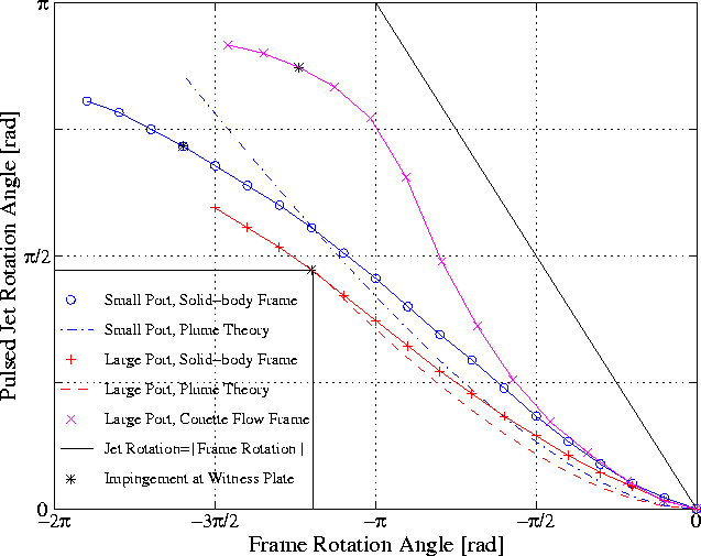
Figure 9: Figure 9 shows the data for the differential rotation of pulsed jets driven from the small port, "o" points and large port, "+" points. Since the differential angle is negative relative to the rotation of the frame, a positive differential angle corresponds to a negative frame angle. The reference frame for two cases is solid-body rotation. The third data are from the Ωdifferential flow similar to Ω ∝ 1/R. The data are derived from the images in Figs. 5, 6, and 12. The magnitude of the measurement error in pulsed jet rotation angle is comparable with the size of the data points. The origin is where the jet pulse and the electrolysis pulse coincide. The two theoretical curves are from Eq. (5) with the dash-dot using the small port parameters and the long-dash curve using the large port parameters. vR<<95>>0 = 48 cm/s, vjet,SP(Ω = const) = 7.5 cm/s, vjet,LP(Ω = const) = 8.3 cm/s, vjet,LP(Ωdifferential) = 8.2 cm/s.
In Fig. 9, the solid line of slope = - 1 represents the maximum possible relative rotation angle in an Ω = const fluid flow. This limiting case is where the pulsed jet assumes infinite expansion and no friction with the rotating reference frame. In this limiting case, with respect to the laboratory reference frame, Δωjet = 0. We calculate the expected differential rotation angle ΔΦjet for each of the port sizes using the average measured vertical jet velocities measured from from Figs. 5 and 6. We observe a radial divergence angle close to a half-angle of = 1/2π, approximately the same as if the laminar flow ahead of the pulsed jet diverges at the same rate as it would under ideal entrainment. The vertical jet velocities remain near constant at 7.5 and 8.3 cm/s for the small and large ports respectively. The approximation for the pulsed jet radius is then
where time t is measured from when the jet emerges from the port at t0 and where rport is the initial radius of the jet as it exits the port in the experiment. Figure 9 also shows the time when the pulsed jets impinge on the witness plate at timpinge beyond which the radius of Eq. (2) no longer applies. The rotation of the jet occurs because of the transient conservation of angular momentum of the flow ahead of the pulsed jet (rather than the jet itself) as it expands radially, relative to its own axis. The expansion leads to an increase in moment of inertia of
Therefore, following such an expansion the rotation rate of the pulsed jet, ωjet relative to the rotation of the frame, Ω0 becomes
We derive the differential rotation angle ΔΦ by substituting Eq. (2) into Eq. (4) for rjet. By integrating over the jet lifetime from t= 0 to t we obtain the expected differential rotation angle, measured in radians, as
where
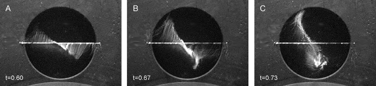
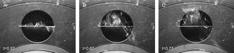
For Ω0 = 2π × 1/2 Hz = π rad/s, one has for the small port Ω0τsp = 4.34 rad, and for the large port Ω0τsp = 5.71 rad. Thus one notes that the frame rotates nearly a full revolution during the rise of the jet. Figure 9 shows the results of the theoretical differential rotation angle, Eq. (5), and the measurements of pulsed jet differential rotation. The data points are connected for visual reference. The theoretical curves are shown dash-dot for the small port with the higher rotation rate and long-dash for the large port with slower rotation rate. We have also drawn a solid straight line as an upper bound on pulsed jet rotation where a stationary jet rotates at Ω0 relative to the frame. One notes that the actual differential pulsed jet rotation is slightly faster than the theory indicating a jet expansion angle slightly greater than the classic plume entrainment half-angle of 1/2π and so a slightly greater differential rotation is expected than the ideal of Eq. (5). We expect the drag to become larger due to the enhanced turbulence when the jet strikes the witness plate. The curvature at the upper end of the experimental curves after striking the witness plate is consistent with this explanation. Note the longer time for the small jet to strike the witness plate because of both the slower velocity and the larger distance from the port to the witness plate: 12.5 cm rather than 10 cm. We have also included the data from the differential frame rotation case of annular rotational Couette flow measurements of Fig. 12. Here the differential rotation angle of the pulsed jet is measured (+π/2 radians) relative to the radial from the axis to the center of mass of the bubbles outlining the jet. This shift accounts for the shift of the pulsed jet relative to the camera axis because of the differential frame rotation. We also note the greater rotation rate of the jet relative to the Ω = const case presumably because of entrainment in the sheared flow. Before discussing the differential frame case, we consider the rotation within the pulsed jet as compared to the rotation of matter pushed ahead of the jet. C. Convergent FlowWe next consider the convergent flow behind the vortex ring forming the head of the jet. This convergent flow is most clearly evident in Fig. 3(C). We expect that this convergent flow, as compared to the divergent flow at the head of the jet, will lead to co-rotation of the jet, opposite to the counter-rotation observed in Figs. 5 and 6. In order to show how the convergent flow affects the pulsed jet rotation we have used a delayed pulse of electrolysis (0.5 s delay, 0.1 s duration), as well as an extended electrolysis pulse (0.5 s duration). The extended electrolysis pulse superposes the convergent flow co-rotation beneath the divergent flow counter-rotation. The equivalent timing of these delayed and extended electrolysis pulses relative to the vertical jet motion are shown in Figs. 3(B) and 3(C) respectively. Both the delayed and extended pulses demonstrate the expected co-rotation of the convergent flow behind the vortex ring as being opposite to the counter-rotation of the divergent flow ahead of the pulsed jet. The delayed pulse of Fig. 10 shows that the base of the jet is co-rotating with the reference frame. Figure 11 shows both rotations superimposed. Note that the convergent flow in Fig. 11 loses its initial coherence more rapidly through turbulent entrainment. The opposite rotation of the convergent flow terminates the effective helicity generated by the jet. Hence, dynamo modeling must include this effect.
Figure 10:
Figure 10 shows the effect of convergent flow at the base
of the pulsed jet in the Ω = const solid-body rotation case.
The delayed electrolysis pulse shows that the base of the jet is
co-rotating with the reference frame (ANIMATE
Figure 11:
Figure 11 exhibits an extended electrolysis pulse showing
an overlay of the counter-rotation of the jet head and the co-rotation
of the jet base (ANIMATE D. Differential Frame RotationWe now consider where the background flow field is in differential rotation, Ωdifferential, as compared to &Omega = const flow. It is more difficult in this case to obtain accurate visualization images for two reasons: (1) the camera is mounted at R0 and therefore rotates at Ω = &Omega0 whereas the jet, although injected at Ω0, soon is swept with the flow to an intermediate value of Ω, and (2) the resulting shear within the flow around the jet and ahead of the jet leads to more rapid entrainment and consequently the dispersal of the "line" of bubbles. As a consequence we chose to use an intermediate flow field where the inner boundary rotates at Ω1 = Ω0(R0/R1). By way of comparison, the maximum stable annular rotational Couette flow which corresponds to Ωdifferential ∝ 1/R will be used in the liquid sodium experiment. If the shear were greater, the flow field becomes unstable with resulting turbulence, large drag, and hence, power loss. Keplerian motion in an accretion disk has somewhat less shear, Ωdisk ∝ 1/R3/2, but more than our choice of Ωdifferential ∝ 1/R. Figure 12 shows the effect on pulsed jet rotation through entrainment with the Ωdifferential background flow. Compared to Figs. 5 and 6, Fig. 12 shows the differential rotation rate of the jet relative to the frame is higher, although the bubble line disperses more rapidly. The quantitative analysis of the pulsed jet for this case is shown in Fig. 9. This greater angular rotation is presumed to be due to the entrainment with the differential rotation of the background flow. If the entrainment were instantaneous in the Ω = 0 rotation case, then no jet rotation would be observed. Conversely, in the case of shear flow with full entrainment but without expansion the rotation of the jet would approximately be the same as the solid line corresponding to infinite expansion and no shear case of Fig. 9. Hence entrainment plays an important, but not dominant role in determining the rotation of the pulsed jet.
Figure 12:
Figure 12 shows the top view showing pulsed jet rotation
in an Ωdifferential fluid flow field (ANIMATE Figure 13 shows how the convergent flow affects the jet rotation in the Ωdifferential case. We used an electrolysis pulse with 0.5 s delay and 0.1 s duration. Figure 13 shows that the converging flow at the base of the jet in the differentially rotating background flow has no further rotation. Since the Ωdifferential flow field enhances the divergent flow counter-rotation characteristic of the jet, it should reduce the co-rotation of the converging flow.
Figure 13:
Figure 13 shows the delayed electrolysis pulse in an
Ωdifferential flow field (ANIMATE |