We first discuss the two classical necessary conditions long thought to be needed for the production of deep convection, conditional instability and a triggering mechanism. We then discuss more recently developed criteria, which attempt to establish both necessary and sufficient conditions for the development of convection.
Figure 6.1 shows a schematic of a conditionally unstable sounding expressed in terms of the moist entropy and the saturated moist entropy plotted as a function of height. Conditional instability means that finite energy must be expended to lift a parcel to the point where it is positively buoyant. The decrease in both saturated and unsaturated moist entropy up to some level, followed by an increase with height is universally found in conditionally unstable soundings.
The saturated moist entropy is the moist entropy with the vapor mixing ratio replaced by the saturated mixing ratio. The moist entropy is conserved in both moist and dry adiabatic processes, so the moist entropy of a surface parcel lifted through the troposphere follows the vertical trajectory shown in figure 6.1. The saturated moist entropy of the surface parcel initially follows a line of constant potential temperature, which low in the troposphere slants sharply to the left, as shown. However, when the saturated entropy line intersects the moist entropy line, the parcel becomes saturated. This level is called the lifting condensation level (LCL). Subsequently the saturated moist entropy equals the moist entropy, so both follow the vertical trajectory of the lifted surface parcel.
Neglecting virtual temperature effects, the difference between the saturated moist entropy of a parcel and its surrounding environment is a measure of the buoyancy of the parcel relative to the environment. Thus, when the saturated moist entropy of the parcel exceeds the saturated moist entropy of the environment, the buoyancy of the parcel, which typically is negative initially, becomes positive. This level is called the level of free convection (LFC). The parcel will eventually reach its level of neutral buoyancy (LNB), after which the buoyancy becomes negative.
The buoyancy of a lifted surface parcel is initially negative relative to the environment (with the exception of a possible shallow region of positive buoyancy over sun-heated land) in almost all cases. Thus, some energy source is required to lift the parcel initially to its level of free convection. The required energy per unit parcel mass is called the convective inhibition (CIN). We now derive an equation for CIN. Realizing that the net buoyancy force consists of the downward force of gravity on the parcel plus the upward pressure force which equals the weight of the displaced parcel of environmental air Me, the work needed to lift the parcel from its initial level (z=zI) to the level of free convection (z=zLFC) is the CIN times the mass of the parcel Mp:
| CIN× Mp= | ∫ |
| g(Mp−Me)dz, (6.1) |
where g is the acceleration of gravity. Dividing by Mp results in
| CIN= | ∫ |
| g(1−ρe/ρp)dz, (6.2) |
where ρp and ρe are the densities of the parcel and the environment.
It is more convenient to express equation (6.2) in the form of a pressure integral, converting from geometrical height to environmental pressure p using the hydrostatic equation dp=−gρedz:
| CIN= | ∫ |
| (1/ρe−1/ρp)dp, (6.3) |
where pI and pLFC are the pressures at the initial level and the level of free convection. Using the equation of state for an air parcel with vapor mixing ratio rV and condensate mixing ratio rC,
| = |
| (1+0.61rV−rC), (6.4) |
we finally get
| CIN=RD | ∫ | [Te(1+0.61rVe)−Tp(1+0.61rVp−rCp)]dlnp, (6.5) |
where a subscripted e indicates environment and a p indicates parcel values. We have assumed that no condensate exists in the environment. The virtual temperature is defined
| TV=T(1+0.61rV−rC), (6.6) |
so the integrand is simply the difference between the virtual temperatures of the environment and the parcel.
A similar integral yielding the energy released per unit mass in a parcel ascending from the level of free convection to the level of neutral buoyancy is called the convective available potential energy (CAPE):
| CAPE=RD | ∫ |
| [Tp(1+0.61rVp−rCp)−Te(1+0.61rVe)]dlnp. (6.7) |
The order of environmental and parcel quantities is reversed in the integrand compared to the expression for CIN, since CAPE is energy released by the parcel ascent, whereas CIN is the external energy required to lift the parcel.
Generally the negative parcel buoyancy resulting in positive CIN for daytime convective environments comes from a stable layer above the lifting condensation level where the parcel is saturated. The specific moist entropy s of the parcel in this case equals the saturated moist entropy ss, which is a function only of the temperature and the pressure as long as the condensed water content is small enough to be neglected. At a given pressure level the difference between the temperature of the parcel and the environment can therefore be related to the difference between the moist entropy of the parcel and the saturated moist entropy of the environment,
| sp−sse=ssp−sse= |
| (Tp−Te), (6.8) |
where the partial derivative of the saturated moist entropy is taken at constant pressure. Thus, to the extent that the difference between real and virtual temperatures can be ignored, the part of the CIN above the lifting condensation level can be written
| CINmoist≈ RD | ∫ |
| ⎛ ⎜ ⎜ ⎝ |
| ⎞ ⎟ ⎟ ⎠ |
| ⎡ ⎣ | sse(p)−sp | ⎤ ⎦ | dlnp. (6.9) |
Similarly, the CAPE can be approximated
| CAPEmoist≈ RD | ∫ |
| ⎛ ⎜ ⎜ ⎝ |
| ⎞ ⎟ ⎟ ⎠ |
| ⎡ ⎣ | sp−sse(p) | ⎤ ⎦ | dlnp. (6.10) |
CAPE and CIN are functions of the characteristics of the convective parcel itself and the environment through which it ascends. Convective parcels are largely produced in the planetary boundary layer, so the characteristics of this layer and the factors controlling it such as surface fluxes and entrainment from the free troposphere are crucial.
Almost all deep convection originates in a layer in the troposphere called the planetary boundary layer (PBL). This is the layer adjacent to the surface in which turbulence acts to mix the layer. Though in practice this mixing is never carried to completion, a useful idealized model of the PBL assumes that the mixing keeps this layer homogenized. Atmospheric motions can distort this layer, increasing or decreasing its thickness and horizontal area. In addition, the PBL generally entrains air from the quiescent free troposphere overlying it.
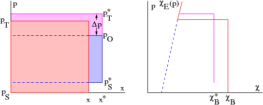
Figure 6.2 shows how a well-mixed intensive variable χ in a control volume might respond to deformations and entrainment which take place over a time interval Δ t, with values at the end of this interval represented by a superscripted asterisk. We assume that the horizontal area of the control volume changes from xy to x*y*. Since the pressure is the weight per unit area of the overlying air, the mass in the initial control volume, with base pressure pS and top pressure pT is xy(pS−pT)/g, where g is the acceleration of gravity. With no entrainment, the control volume neither gains nor loses mass. If pS* is the base pressure after the elapse of the interval and pO is the pressure the top would have had at this point in the absence of entrainment, then conservation of mass tells us that
| xy(pS−pT)/g=x*y*(pS*−pO)/g. (6.11) |
Because of entrainment, the actual top of the PBL is pT*=pO−Δ p at the end of the interval, meaning that the mass in the control volume has increased by approximately xyΔ p/g during the interval.
We assume that the initial value of χ in the control volume is χB and its final value is χB*, while the value in the free troposphere just above the control volume is χE. If χ has an internal source per unit mass per unit time of Sχ and a surface flux per unit area per unit time Fχ, then we can compute χB* assuming that it is the mass-weighted average of the pre-existing value in the control volume and the value in the entrained air plus modifications due to the surface flux and the source term:
| = |
| + |
| +xyFχΔ t. (6.12) |
Letting Δ t→0 and invoking equation (6.11) results in the governing equation for χB,
| = |
| + |
| ωE+Sχ, (6.13) |
where
| ωE= |
|
| (6.14) |
is the entrainment velocity.
Defining the area A=xy and A*=x*y*, we note that pT*=pO−Δ p, and that pS*−pO=(pS−pT)A/A*≈(pS−pT)(1−Δ A/A), where Δ A=A*−A. From this we can determine the thickening rate of the PBL in pressure coordinates,
| =−(pS−pT) |
| +ωE. (6.15) |
If we define the horizontal flow velocity in the PBL as vB, then it is easily demonstrated that
| =∇h·vB (6.16) |
where ∇h is the two-dimensional horizontal gradient operator.
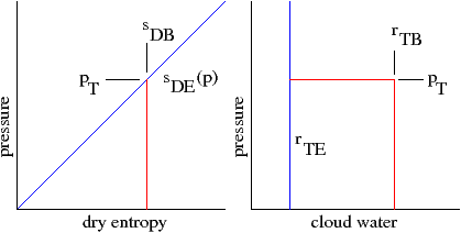
Figure 6.3: Growing cloud-free PBL resulting from surface dry entropy and water vapor fluxes. The dry entropy of the PBL, sDB, matches the dry entropy of the environment, sDE, at PBL top pT.
We now analyze an example to illustrate how these equations are applied. For this example we assume that dlnA/dt=0. Figure 6.3 illustrates a cloud-free PBL in an environment with a linear environmental profile of dry entropy sDE=Γ(pS−pT) (which is conserved in the non-condensing case) and a constant environmental mixing ratio rTE of total cloud water. Constant surface fluxes of dry entropy Fs and water vapor Fr are specified and possible source terms (such as radiation for entropy) are ignored. As is observed in developing boundary layers in light winds, the value of dry entropy in the PBL closely matches the environmental value at PBL top. Under these conditions equation (6.13) reduces to
| = |
| , (6.17) |
for the dry entropy and to
| = |
| + |
| ωE (6.18) |
for the mixing ratio.
The condition on dry entropy at the top of the PBL leads to
| sDB=Γ(pS−pT). (6.19) |
Using this to eliminate pS−pT in equation (6.17) leads to a simple differential equation for sDB which has the solution
| sDB=(2gFsΓ t)1/2. (6.20) |
Thus, the entropy of the PBL increases with the square root of time, as does the thickness of the PBL.
The entrainment velocity equation in this case can be obtained from equation (6.15):
| ωE= |
| = | ⎛ ⎜ ⎜ ⎝ |
| ⎞ ⎟ ⎟ ⎠ |
| = |
| . (6.21) |
The moisture equation (6.18) is slightly more difficult to solve. However, the substitution rTB−rTE=η/t1/2 leads to a solution in terms of η, which upon re-expression in terms of rTB is
| rTB=rTE− |
| + |
| ⎛ ⎜ ⎜ ⎝ | 1− |
| ⎞ ⎟ ⎟ ⎠ | (6.22) |
where r0 is the total water mixing ratio in the PBL at the time
| t0= |
| , (6.23) |
and where Δ p0=pS−pT is the PBL thickness at this time. Defining the dimensionless PBL thickness σ=(pS−pT)/Δ p0, the PBL mixing ratio equation simplifies to
| rTB= |
| + | ⎛ ⎜ ⎜ ⎝ |
| ⎞ ⎟ ⎟ ⎠ | ⎛ ⎜ ⎜ ⎝ |
| ⎞ ⎟ ⎟ ⎠ | . (6.24) |
Thus, the PBL mixing ratio is controlled by competing mechanisms which respectively tend to increase and decrease the mixing ratio as the PBL thickens by entrainment. The first term in this equation tends to decrease the mixing ratio with increasing thickness as long as rTE<r0, i. e., when the initial boundary layer mixing ratio exceeds that of the environment. This decrease is due simply to the entrainment of drier air from above the PBL. The second term increases with time at a rate which is proportional to the surface moisture flux. Thus, the surface moisture flux must exceed a certain critical value for the mixing ratio of the PBL to increase with time. Over land, the moisture flux depends strongly on the wetness of the soil and on the transpiration rate of vegetation.
Recall that a key parameter in the development of deep convection is the PBL moist entropy. We can combine equation (6.19), written sDB=ΓΔ p0σ, and equation (6.24) to get the simplified form of the moist entropy s=sD+LrV/TF in the PBL, assuming that the PBL remains unsaturated so that rV=rT:
| sB=ΓΔ p0 | ⎡ ⎢ ⎢ ⎣ | σ+ |
| ⎛ ⎜ ⎜ ⎝ |
| ⎞ ⎟ ⎟ ⎠ | ⎤ ⎥ ⎥ ⎦ | + |
| , (6.25) |
where the dimensionless quantity
| B= |
| (6.26) |
is called the Bowen ratio. The Bowen ratio is the ratio of sensible to latent heat transfer to the atmosphere from the surface.
Entrainment of dry air from above the PBL tends to decrease the PBL moist entropy in the above formulation. This is manifested in the second term on the right side of equation (6.25), which asymptotically drives the mixing ratio to the free tropospheric value for large σ. Surface moisture fluxes can counteract this if they are large enough relative to the surface heat fluxes. This eventuality is manifested by a small Bowen ratio. Since the development of deep convection requires sB to exceed a certain threshold, the importance of surface moisture fluxes (i. e., evaporation from the surface) cannot be overemphasized. This can lead to positive feedback: if the ground is already moist, more convection and precipitation is likely to occur. However, if the ground is dry, deep convection and precipitation are inhibited.
Scaling arguments originating with G. I. Taylor give us equations for surface fluxes of entropy, moisture, and momentum. For an intensive variable χ, with PBL value χB, the surface-air flux is approximately
| Fχ=ρsCE(χss−χB)Ueff, (6.27) |
where ρs is the air density at the sea surface, CE≈1×10⁻³ is an exchange coefficient, and χss is the value of χ for air in immediate contact with the surface. The quantity Ueff is the effective surface wind speed,
| Ueff=(UB2+W2)1/2, (6.28) |
where UB is the mean PBL wind speed and W is a parameter which accounts for the averaged effect of PBL wind variability, which is important in low wind situations. Typically we find that W≈3 m s−1. The exchange coefficient CE is a function of the atmospheric static stability near the surface, with instability leading to larger values of CE. If strong stability exists in this layer, then CE becomes small, effectively shutting off the fluxes.
Surface fluxes of three variables are of particular importance, entropy, water vapor, and momentum. Over the ocean, the values of χss are well-defined for each of these variables. For entropy and water vapor, χss equals respectively the saturated moist entropy and saturation mixing ratio at the temperature and pressure of the sea surface. For momentum, it equals the velocity of the sea surface, generally close to zero. Over land as well as over the ocean, the momentum flux depends on a parameter called the roughness length (see Stull, 1988), which has an effect on the value of CE.
Determination of the entropy and moisture fluxes over land is more difficult than over the ocean. The quantity χss cannot be specified as easily as it can over the ocean. Instead, the usual approach is to compute explicitly the budget of heat and moisture in the soil as a function of depth. A byproduct of this approach is the surface fluxes of these quantities. A complicating factor over land is the role of vegetation in transporting moisture from beneath the land surface into the atmosphere. This leads to a large role for biological mechanisms in the surface moisture flux over land.
Geographical inhomogeneities such as topography and variability in surface properties can cause certain regions to be more favorable to the initiation of deep convection. Obvious cases of this convective focusing are the initiation of convection due to the elevated heating of the morning sun on high terrain, and differential solar heating at the land-sea boundary. The net effect in these cases is to modify locally the depth, entropy, and mixing ratio of the PBL, leading to strong local variations in CAPE and CIN. Typically, deep convection forms in regions in which the PBL has become locally thickened, as this thickening has the effect of reducing the convective inhibition. The thickened region of the PBL may also exhibit larger moist entropy, which also reduces CIN and increases CAPE as well.
Geophysical fluid dynamics GFD tells us how the large-scale flow works in the earth’s atmosphere. Consideration of this topic is beyond the scope of the course, but the essential point is that GFD exerts a strong control over the wind and temperature profiles in the free troposphere. Thus, the free tropospheric contribution to CAPE and CIN is largely determined by GFD. The interaction between the large-scale flows governed by GFD and the collective behavior of convection is a fascinating topic which we don’t have time to discuss here. Large-scale flows also govern (together with convection itself) the distribution of moisture in the atmosphere. The distribution of moisture is of great import to convection.
One aspect of large-scale forcing can be discussed here, namely the effect of large-scale pressure gradients imposed from aloft on the PBL. One of the problems posed below addresses the issue of Ekman balance in the PBL – a situation in which a local balance exists between pressure gradient, Coriolis, and surface drag forces. The actual PBL flow is often not too far from that prescribed by Ekman balance, though recent work suggests that incorporation of the momentum fluxes from air entrained from the free troposphere is necessary for reasonable accuracy in some instances. Convergence in the Ekman balance flow results in thickening of the PBL and possible destabilization to deep convection.
According to the classical picture of convective initiation, convection occurs when sufficient convective available potential energy exists and when the convective inhibition is locally reduced to the point at which a convective parcel can be lifted to the level of free convection by mechanical processes acting in the PBL. Though it is clear that the combination of these two conditions generally produces moist convection, it is not obvious that the resulting convection will be either deep or precipitating, and in most cases it is neither.
The educated eye tells one that deep convection rarely if ever develops directly out of the PBL as conventionally defined, but rather forms from an extensive mass of pre-existing shallow cumulus clouds. These clouds may start out as the well-mixed top of a PBL. However, as they grow, the entrainment of free tropospheric air causes the mean conditions in the cloud layer to deviate significantly from being well-mixed with the underlying subcloud layer. The dynamics of this cloud layer is like that of the mixing layer envisioned by Frasier (1968) or Raymond and Blyth (1986).
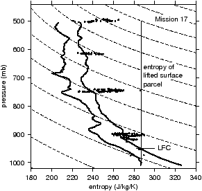
Figure 6.4 shows that values of moist entropy inside a deep convective cloud over the tropical east Pacific do not approach those of the sub-cloud layer, but are characteristic of parcels originating from as high as 800 hPa. This result is typical of measurements in many tropical oceanic clouds as well as those which form over land.
The energy for the mixing in the mixing layer comes from the fact that the moist entropy decreases with height in this layer (see figure 6.1). If the mixing layer is saturated, then the reference profile for static stability is one with constant moist entropy. If the moist entropy decreases with height in this layer, then a vertically displaced moist parcel will acquire a buoyancy which causes it to accelerate away from its initial level. Numerical models of deep moist convection show little evidence of entrainment of environmental air by deep convective thermals at levels above the level of minimum environmental moist entropy.
The mechanism by which deep convective thermals form out of cloudy air in the mixing layer is shrouded in mystery. Such thermals must typically be large enough to ascend to great altitude without experiencing significant entrainment of environmental air. Is the development of such a thermal out of a turbulent field simply the result of a statistical accident? Does the successful thermal gain an advantage by commencing the production of precipitation, leaving less liquid water to cause evaporative cooling upon mixing with environmental air? Does the initiation of ice nucleation lead to additional heating which is crucial to overcoming the CIN? Many such questions remain to be answered.
Evidence is accumulating that deep convection is harder to produce and sustain in environments with low rather than high relative humidity, irrespective of the value of CAPE in the environmental sounding. This is consistent with the idea that evaporative cooling upon mixing with dry air is detrimental to the production of deep convection. However, it is not known whether the mixing in question is of greatest importance in the mixing layer, or whether the dry air saps the thermal primarily after it leaves the mixing layer.
If precipitation falls out of a cloud into dry air, it will begin to evaporate. This evaporation cools the air, resulting in the formation of a precipitation-induced downdraft. (The weight of the precipitation can by itself cause an air parcel to sink, but this negative buoyancy is reversed as soon as the precipitation falls out of the parcel.) In a layer in which the saturated moist entropy decreases with height, the cooled parcel actually gains capacity to absorb evaporated water as it descends to maintain buoyancy equilibrium with its surroundings.
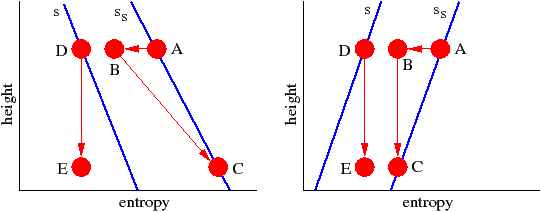
This phenomenon is shown in figure 6.5. Cooling a parcel at constant height corresponds to moving it to the left in the entropy-height plane, i. e., from point A to point B. The moist entropy of the parcel remains unchanged during this cooling. Since the parcel now has negative buoyancy, it sinks, with the saturated moist entropy following a constant potential temperature line BC. Sinking terminates when the saturated moist entropy of the parcel matches that of the environment. At this level the parcel is again in buoyancy equilibrium with the environment. The moist entropy of the parcel doesn’t change in these two processes, which means that the trajectory of the parcel’s moist entropy is vertical, DE.
Notice that the difference between moist entropy and saturated moist entropy decreases when the saturated moist entropy increases with height (right panel of figure 6.5), and increases when the saturated moist entropy decreases with height (left panel). The latter generally occurs in the lower part of the free troposphere. An increase in this difference makes precipitation evaporate more readily, whereas a decrease causes evaporation to be slower. Thus, in the lower troposphere where saturated moist entropy decreases with height, sinking due to evaporation of precipitation is a runaway process which accelerates as the parcel sinks in the presence of precipitation, while the reverse is true in the upper troposphere, where the saturated moist entropy increases with height. In the latter case, if the moist entropy of the parcel exceeds the saturated moist entropy of the environment at some level, the parcel cannot sink beyond that level. This implies that downdrafts reaching the surface originate primarily from the level of minimum saturated moist entropy and below.
So far we have discussed the possible production of deep convection from the PBL. However, we have not yet discussed the feedbacks imposed on the PBL by deep convection. The most important feedbacks appear to be the extraction of updraft mass from the PBL and its partial replacement by downdraft air. Equation (6.11) representing mass conservation in the PBL becomes
| xy(pS−pT)/g−xy(Mu−Md)Δ t=x*y*(pS*−pO)/g (6.29) |
when this is accounted for, where Mu and Md are the mass per unit area per unit time extracted from and returned to the PBL by deep convection. Similarly, the governing equation (6.13) for an intensive variable χ generalizes to
| = |
| + |
| + |
| ωE+Sχ (6.30) |
where χd is the value of χ in convective downdrafts, while equation (6.15) becomes
| =−(pS−pT) |
| +g(Mu−Md)+ωE (6.31) |
(see Raymond 1995).
The transports of entropy, moisture, and momentum into the PBL by deep convection can have major effects on the PBL. This subject lies at a sub-discipline boundary in the atmospheric sciences, and thus has not received the attention it deserves.
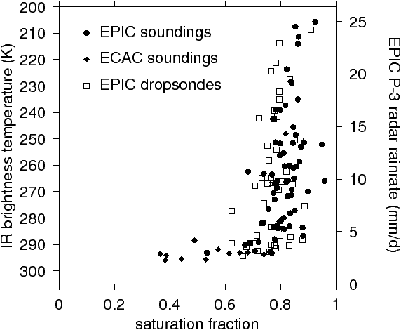
Figure 6.6: Saturation fraction as a function of satellite infrared brightness temperature and inferred precipitation rate in the tropical east Pacific and the southwest Caribbean.
Just because there is moist convection does not necessarily mean that rainfall occurs. The convection may occur in an environment which is so dry that entrainment evaporates most of the condensed water. Alternatively, precipitation which does form may fall into a deep, dry boundary layer where it evaporates.
Recent work over the tropical oceans (Bretherton, Peters, and Back 2004) shows a high correlation between the rainfall rate averaged over areas of order a few square degrees and the saturation fraction, defined as
| F≡ | ∫ |
| rVdp | / / / / / / | ∫ |
| rSdp | (6.32) |
where ps is the surface pressure and rV and rS are the water vapor mixing ratio and the saturation mixing ratio. The saturation fraction is a kind of column-integrated relative humidity. Alternatively, it may be thought of as the ratio of precipitable water to saturated precipitable water. Figure 6.6 shows an example of this relationship over the eastern tropical Pacific and the southwest Caribbean sea. The applicability of this relationship over land has yet to be determined.
A vast amount of work has been done in characterizing the morphology of convective systems. This work is well described by Houze (1993) and is treated very briefly here.
A typical thunderstorm cell typically produces an initial gush of heavy rain, with the intensity of the rain decreasing gradually over an extended period. Multiple cells in an organized system can produce an extended middle to upper tropospheric layer of stratiform cloud which extends the lifetime and amount of this tail of light rain. A formal distinction has been made between convective rain (the early period of heavy rain) and stratiform rain (the extended tail of light rain). The distinction is an empirical one, but it has some physical basis. The heavy rain is typically the result of heavy riming of ice crystals that fall back through the supercooled water in the cell’s updraft. The light stratiform rain generally consists of ice crystals which have been blown out of the top of the updraft into an upper level stratiform layer, where they aggregate into snow flakes. They then fall out of the stratiform cloud, melting at the freezing level and thus turning into small raindrops.
Radar observations of stratiform rain commonly show a bright band at the freezing level, i. e., a thin layer of elevated radar reflectivity at this level. This is produced by melting snowflakes which have yet to acquire the higher terminal velocity of raindrops, but have developed higher reflectivity due to the partial melting and development of a surface layer of liquid water. This bright band does not exist in the region of convective rain, because the falling precipitation particles are of higher density and fall speed, and thus melts over a much broader vertical range.
Low-entropy downdrafts produced by evaporating precipitation spread out in the form of gust fronts when they reach the surface. These gust fronts propagate across the surface, sometimes lifting surrounding PBL air to the level of free convection, thus producing new deep convective cells. If the vertical shear of the horizontal wind is weak, this production of cells and proliferation of gust fronts is somewhat random and disorganized. It basically proceeds until the high-entropy PBL air is exhausted, or at least until the swarm of gust fronts is unable to lift the remaining conditionally unstable air to the level of free convection. Such convection is thus autocatalytic to a certain degree, with the initial round of convective cells contributing to the development of others.
When significant wind shear exists in the troposphere, especially in the lowest few kilometers, the lifting of undisturbed PBL air to the level of free convection becomes most efficient on the down-shear side of the downdraft pools of cool air. This can lead to the development of squall lines which propagate downshear, resulting in highly organized, intense convective systems. An extensive literature exists on the morphology and dynamics of squall lines. See in particular the books of Houze (1993) and Emanuel (1994) for more information.
When the shear is strong enough and the convective available potential energy is large, squall lines give way to a type of self-propagating system called a supercell storm. These systems develop cyclonic rotation as the result of incorporating air into updrafts with significant streamwise vorticity. The rotation acts dynamically to cause uplift on one of the flanks of the storm, generally the right flank (facing down-shear) in the northern hemisphere. Houze (1993) describes the propagation mechanism of supercell storms.
These storms are the most violent local storms that occur, and frequently have large hail and strong tornadoes associated with them.
This document was translated from LATEX by HEVEA.