A Radically Modern Approach to Introductory Physics
Second Edition
Volume 2: Four Forces
David J. Raymond
The New Mexico Tech Press
Socorro, New Mexico, USA
A Radically Modern Approach to Introductory Physics Second Edition
Volume 2: Four Forces
David J. Raymond
Copyright © 2012, 2015 David J. Raymond
Second Edition
Original state, 14 December 2015
Content of this book available under the Creative Commons Attribution-Noncommercial-Share-Alike License. See http://creativecommons.org/licenses/by-nc-sa/3.0/ for details.
Publisher’s Cataloging-in-Publication Data
OCLC Number: 932065971 (print) – 932066146 (ebook)
Published by The New Mexico Tech Press, a New Mexico nonprofit corporation
This copy printed by CreateSpace, Charleston, SC
Printed in the United States of America
The New Mexico Tech Press
Socorro, New Mexico, USA
http://press.nmt.edu
To my wife Georgia and my daughters Maria and Elizabeth.
The idea for a “radically modern” introductory physics course arose out of frustration in the physics department at New Mexico Tech with the standard two-semester treatment of the subject. It is basically impossible to incorporate a significant amount of “modern physics” (meaning post-19th century!) in that format. It seemed to us that largely skipping the “interesting stuff” that has transpired since the days of Einstein and Bohr was like teaching biology without any reference to DNA. We felt at the time (and still feel) that an introductory physics course for non-majors should make an attempt to cover the great accomplishments of physics in the 20th century, since they form such an important part of our scientific culture.
It would, of course, be easy to pander to students – teach them superficially about the things they find interesting, while skipping the “hard stuff”. However, I am convinced that they would ultimately find such an approach as unsatisfying as would the educated physicist. What was needed was a unifying vision which allowed the presentation of all of physics from a modern point of view.
The idea for this course came from reading Louis de Broglie’s Nobel Prize address.1 De Broglie’s work is a masterpiece based on the principles of optics and special relativity, which qualitatively foresees the path taken by Schrödinger and others in the development of quantum mechanics. It thus dawned on me that perhaps optics and waves together with relativity could form a better foundation for all of physics, providing a more interesting way into the subject than classical mechanics.
Whether this is so or not is still a matter of debate, but it is indisputable that such a path is much more fascinating to most college students interested in pursuing studies in physics — especially those who have been through the usual high school treatment of classical mechanics. I am also convinced that the development of physics in these terms, though not historical, is at least as rigorous and coherent as the classical approach.
After 15 years of gradual development, it is clear that the course failed in its original purpose, as a replacement for the standard, one-year introductory physics course with calculus. The material is way too challenging, given the level of interest of the typical non-physics student. However, the course has found a niche at the sophomore level for physics majors (and occasional non-majors with a special interest in physics) to explore some of the ideas that drew them to physics in the first place. It was placed at the sophomore level because we found that having some background in both calculus and introductory college-level physics is advantageous for most students. However, we allow incoming freshmen into the course if they have an appropriate high school background in physics and math.
The course is tightly structured, and it contains little or nothing that can be omitted. However, it is designed to fit into two semesters or three quarters. In broad outline form, the structure is as follows:
A few words about how I have taught the course at New Mexico Tech are in order. As with our standard course, each week contains three lecture hours and a two-hour recitation. The recitation is the key to making the course accessible to the students. I generally have small groups of students working on assigned homework problems during recitation while I wander around giving hints. After all groups have completed their work, a representative from each group explains their problem to the class. The students are then required to write up the problems on their own and hand them in at a later date. The problems are the key to student learning, and associating course credit with the successful solution of these problems insures virtually 100% attendance in recitation.
In addition, chapter reading summaries are required, with the students urged to ask questions about material in the text that gave them difficulties. Significant lecture time is taken up answering these questions. Students tend to do the summaries, as they also count for their grade. The summaries and the questions posed by the students have been quite helpful to me in indicating parts of the text which need clarification.
The writing style of the text is quite terse. This partially reflects its origin in a set of lecture notes, but it also focuses the students’ attention on what is really important. Given this structure, a knowledgeable instructor able to offer one-on-one time with students (as in our recitation sections) is essential for student success. The text is most likely to be useful in a sophomore-level course introducing physics majors to the broad world of physics viewed from a modern perspective.
I freely acknowledge stealing ideas from Edwin Taylor, John Archibald Wheeler, Thomas Moore, Robert Mills, Bruce Sherwood, and many other creative physicists, and I owe a great debt to them. The physics department at New Mexico Tech has been quite supportive of my efforts over the years relative to this course, for which I am exceedingly grateful. Finally, my humble thanks go out to the students who have enthusiastically (or on occasion unenthusiastically) responded to this course. It is much, much better as a result of their input.
My colleagues Alan Blyth, David Westpfahl, Ken Eack, and Sharon Sessions were brave enough to teach this course at various stages of its development, and I welcome the feedback I have received from them. Their experience shows that even seasoned physics teachers require time and effort to come to grips with the content of this textbook!
The reviews of Allan Stavely and Paul Arendt in conjunction with the publication of this book by the New Mexico Tech Press have been enormously helpful, and I am very thankful for their support and enthusiasm. Penny Bencomo and Keegan Livoti taught me a lot about written English with their copy editing.
David J. Raymond
Aside from numerous corrections, clarifications, and minor enhancements, the main additions to this edition include the following:
As in the first edition, I am greatful for the reviews of Paul Arendt and Allan Stavely, who always manage to catch things that I have overlooked.
David J. Raymond
Physics Department
New Mexico Tech
Socorro, NM, USA
djraymondnm@gmail.com
In this chapter we study the law that governs gravitational forces between massive bodies. We first introduce the law and then explore its consequences. The notion of a test mass and the gravitational field is developed, followed by the idea of gravitational flux. We then learn how to compute the gravitational field from more than one mass, and in particular from extended bodies with spherical symmetry. We finally examine Kepler’s laws and learn how these laws and the conservation laws for energy and angular momentum may be used to solve problems in orbital dynamics.
Of Newton’s accomplishments, the discovery of the universal law of gravitation ranks as one of the greatest. Imagine two masses, M1 and M2, separated by a distance r. The force has the magnitude
|
| (13.1) |
where G = 6.67 × 10⁻¹¹ m3 kg-1 s-2 is the universal gravitational constant. The gravitational force is always attractive and it acts along the line of centers between the two masses.
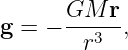
The gravitational field at any point is equal to the gravitational force on some test mass placed at that point divided by the mass of the test mass. The dimensions of the gravitational field are length over time squared, which is the same as acceleration. For a single point mass M (other than the test mass), Newton’s law of gravitation tells us that
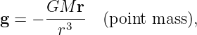 | (13.2) |
where r is the position of the test point relative to the mass M. Note that we have written this equation in vector form, reflecting the fact that the gravitational field is a vector. Thus, r = xtest - xmass, where xtest and xmass are the position vectors of the test point and the mass M. The vector r points from the mass to the test point. The quantity r = |r| is the distance from the mass to the test point.
____________________________
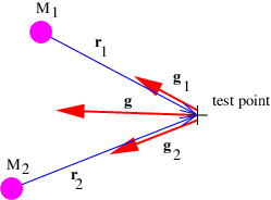
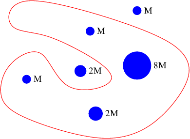
If there is more than one mass, then the total gravitational field at a test point is obtained by computing the individual fields produced by each mass at the test point and vectorially adding these fields. This process is schematically illustrated in figure 13.1.
____________________________
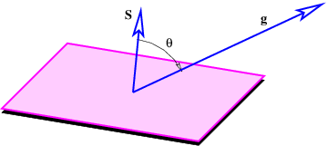
The next concept we need to discuss is the gravitational flux. Figure 13.2 shows a rectangular area S with a vector S perpendicular to the rectangle. The vector S is defined to have length S, so it is a compact way of representing the size and orientation of a rectangle in three dimensional space. The vector S could point either upward or downward, and the choice of directions turns out to be important. This is why we say that S represents a directed area.
Figure 13.2 also shows a vector g, representing the gravitational field on the surface of the rectangle. Its value is assumed here not to vary with position on the rectangle. The angle θ is the angle between the vectors S and g.
____________________________
The gravitational flux through the rectangle is defined as
 | (13.3) |
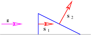
where gn = g cos θ is the component of g normal to the rectangle. The flux is thus larger for larger areas and for larger gravitational fields. However, only the component of the gravitational field normal to the rectangle (i. e., parallel to S) counts in this calculation. A consequence is that the gravitational flux through area 1, S1 ⋅ g, in figure 13.3 is the same as the flux through area 2, S2 ⋅ g.
The significance of the directedness of the area is now clear. If the vector S pointed in the opposite direction, the flux would have the opposite sign. When defining the flux through a rectangle, it is necessary to define which way the flux is going. This is what the direction of S does — a positive flux is defined as going from the side opposite S to the side of S.
An analogy with flowing water may be helpful. Imagine a rectangular channel of cross-sectional area S through which water is flowing at velocity v. The flux of water through the channel, which is defined as the volume of water per unit time passing through the cross-sectional area, is Φw = vS. The water velocity takes the place of the gravitational field in this case, and its direction is here assumed to be normal to the rectangular cross-section of the channel. The field thus expresses an intensity (e. g., the velocity of the water or the strength of the gravitational field), while the flux expresses an amount (the volume of water per unit time in the fluid dynamical case). The gravitational flux is thus the amount of some gravitational influence, while the gravitational field is its strength. We now try to more clearly understand to what this amount really refers.
We need to briefly consider the case in which the gravitational field varies from one point to another on the rectangular surface. In this case a proper calculation of the flux through the surface cannot be made using equation (13.3) directly. Instead, we must break the surface into a grid of sub-surfaces. If the grid is sufficiently fine, the gravitational field will be nearly constant over each sub-surface and equation (13.3) can be applied separately to each of these. The total flux is then the sum of all the individual fluxes.
____________________________
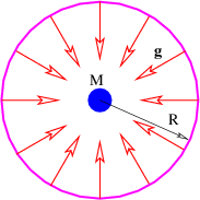
There is actually no need for the area in figure 13.2 to be rectangular. We can calculate the gravitational flux through the surface of a sphere of radius R with a mass M at the center. As illustrated in figure 13.4, the gravitational field points inward toward the mass. It has magnitude g = GM∕R2, so if we desire to calculate the gravitational flux out of the sphere, we must introduce a minus sign. Finally, the area of a sphere of radius R is S = 4πR2, so the flux is
 | (13.4) |
Notice that this flux doesn’t depend on how big the sphere is — the factor of R2 in the area cancels with the factor of 1∕R2 in the gravitational field. This is a hint that something profound is going on. The size of the surface enclosing the mass is unimportant, and neither is its shape — the answer is always the same — the gravitational flux outward through any closed surface surrounding a mass M is just Φg = -4πGM! This is an example of Gauss’s law applied to gravity.
____________________________
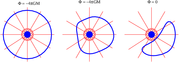
It is possible to formally prove this result using arguments like those posed in figure 13.3, but perhaps the easiest way to understand this result is via the analogy with the flow of water. If we think of the mass as something which destroys water at a certain rate, then there must be an inward flow of water through the surfaces in the left and center examples in figure 13.5. Furthermore, the volume of water per unit time flowing inward through these surfaces is the same in the two examples, because the rate at which water is being destroyed is the same. In the right case the mass is not contained inside the surface and though water flows into the volume bounded by the surface, it also flows out the other side, resulting in a net outward (or inward) volume flux through the surface of zero.
____________________________
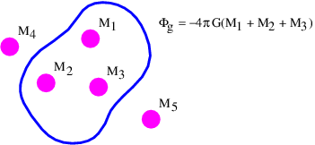
Gauss’s law extends trivially to more than one mass. As figure 13.6 shows, the outward flux through a closed surface is just
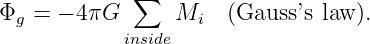 | (13.5) |
In other words, all masses inside the closed surface contribute to the flux, while no masses outside the surface contribute. This is the most general statement of Gauss’s law as it applies to gravity.
An important application of Gauss’s law is to show that the gravitational field outside of a spherically symmetric extended mass M is exactly the same as if all the mass were concentrated at a point at the center of the sphere. The proof goes as follows: Imagine a sphere concentric with the center of the extended mass, but with larger radius. The gravitational flux from the mass is just Φg = -4πGM as before. However, because of the assumed spherical symmetry, we know that the gravitational field points normally inward at every point on the spherical surface and is equal in magnitude everywhere on the sphere. Thus we can infer that Φg = -4πR2g, where R is the radius of the sphere and g is the magnitude of the gravitational field at radius R. From these two equations we immediately infer that the field magnitude is
 | (13.6) |
Expressing this in vector form for arbitrary radius r, and remembering that the gravitational field points inward, we find that
 | (13.7) |
which is precisely the equation for g resulting from a point mass M. Recall that r points from the mass to the test point.
So far our discussion of gravity has been completely non-relativistic. We will not explore in detail how the theory of gravity changes in a completely relativistic treatment. As we noted earlier in the course, Einstein’s general theory of relativity covers this, and the mathematics are formidable. We confine ourselves to two comments:
____________________________
One potentially observable prediction of relativity is the existence of gravitational waves. Imagine two stars revolving around each other. The gravitational field from these stars will change periodically due to this motion. However, this change propagates outward only at the speed of light. As a result, ripples in the field, or gravitational waves, spread outward from the revolving stars. Efforts are currently under way to develop apparatus to detect gravitational waves produced by violent cosmic events such as the explosion of a supernova.
Johannes Kepler, using data compiled by Tycho Brahe, inferred three laws governing the motions of planets in the solar system:
These laws were instrumental in the development of modern mechanics and the universal law of gravitation by Isaac Newton.
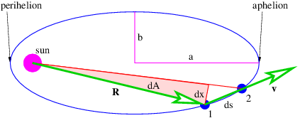
Showing that the first law is consistent with Newtonian mechanics is mathematically more difficult than we can undertake in this course. However, the second law turns out to be a simple consequence of the conservation of angular momentum. Figure 13.7 shows an elliptical orbit with the area swept out as a planet moves from position 1 to position 2. We estimate this area as dA = Rdx∕2, where we have ignored the small unshaded part of the area to the right of the shaded triangle. The distance traveled by the planet in time dt is ds, so the magnitude of the velocity is v = ds∕dt. However, in computing the angular momentum, we need the tangential component of the velocity, i. e., the component normal to the radius vector R. This is simply vt = dx∕dt. The angular momentum is L = mRvt = mRdx∕dt, where m is the mass of the planet. Combining this with the formula for dA results in
 | (13.8) |
Since gravitation is a central force, angular momentum is conserved, which means that dA∕dt is constant. Thus, we have shown that conservation of angular momentum is equivalent to Kepler’s second law.
Kepler’s third law turns out to be a consequence of the universal law of gravitation. We can prove this for circular orbits. We know that a planet moving in a circular orbit around the sun is accelerating toward the sun with the centripetal acceleration a = v2∕R, where v is the speed of the planet’s motion in its orbit and R is the orbit’s radius. This acceleration is caused by the gravitational force, so we can equate the force divided by the planetary mass to a, resulting in
 | (13.9) |
where M is the mass of the sun. This may be solved for v:
 | (13.10) |
Eliminating v in favor of the period of revolution T = 2πR∕v results in
 | (13.11) |
This agrees with Kepler’s third law since the semi-major axis of a circle is simply the radius R.
The gravitational force is conservative, so two point masses M and m separated by a distance r have a potential energy:
 | (13.12) |
It is easily verified that differentiation recovers the gravitational force.
____________________________
The conservation of energy and angular momentum in planetary motions can be used to solve many practical problems involving motion under the influence of gravity. For instance, suppose a bullet is shot straight upward from the surface of the moon. One might ask what initial velocity is needed to insure that the bullet will escape from the gravity of the moon. Since total energy E is conserved, the sum of the initial kinetic and potential energies must equal the sum of the final kinetic and potential energies:
 | (13.13) |
For the bullet to escape the moon, its kinetic energy must remain positive no matter how far it gets from the moon. Since the potential energy is always negative, asymptoting to zero at infinite distance (i. e., Ufinal = 0), the minimum total energy consistent with this condition is zero. For zero total energy we have
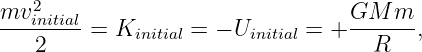 | (13.14) |
where m is the mass of the bullet, M is the mass of the moon, R is the radius of the moon, and vinitial is the minimum initial velocity required for the bullet to escape. Solving for vinitial yields
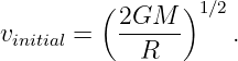 | (13.15) |
This is called the escape velocity. Notice that the escape velocity from a given radius is a factor of 21∕2 larger than the velocity needed for a circular orbit at that radius (see equation (13.10)).
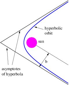
An object is energetically bound to the sun if its kinetic plus potential energy is less than zero. In this case the object follows an elliptical orbit around the sun as shown by Kepler. However, if the kinetic plus potential energy is zero, the object follows a parabolic orbit, and if it is greater than zero, a hyperbolic orbit results. In the latter two cases the sun also resides at a focus of the parabola or hyperbola. Figure 13.8 shows a typical hyperbolic orbit. The impact parameter, defined in this figure, is the closest the object would have come to the center of the sun if it hadn’t been deflected by gravity.
Sometimes energy and angular momentum conservation can be used together to solve problems. For instance, suppose we know the energy and angular momentum of an asteroid of mass m and we wish to infer the maximum and minimum distances of the asteroid from the sun, the so-called aphelion and perihelion distances. Since the asteroid is gravitationally bound to the sun, it is convenient to characterize the total energy by Eb = -E, the so-called binding energy. If v is the orbital speed of the asteroid and r is its distance from the sun, then the binding energy can be written in terms of the kinetic and potential energies:
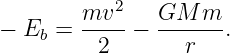 | (13.16) |
The magnitude of the angular momentum of the asteroid is L = mvtr, where vt is the tangential component of the asteroid’s velocity. At aphelion and perihelion, the radial part of the velocity of the asteroid is zero and the speed equals the tangential component of the velocity, v = vt. Thus, at aphelion and perihelion we can eliminate v in favor of the angular momentum:
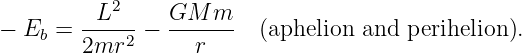 | (13.17) |
This can be rearranged into a quadratic equation
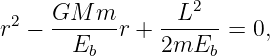 | (13.18) |
which can be solved to yield
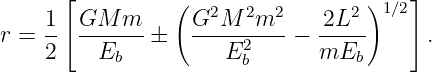 | (13.19) |
The larger of the two solutions yields the aphelion value of the radius while the smaller yields the perihelion.
Equation (13.19) tells us something else interesting. The quantity inside the square root cannot be negative, which means that we must have
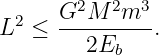 | (13.20) |
In other words, for a given value of the binding energy Eb there is a maximum value for the angular momentum. This maximum value makes the square root zero, which means that the aphelion and the perihelion are the same — i. e., the orbit is circular. Thus, among all orbits with a given binding energy, the circular orbit has the maximum angular momentum.
_____________________________________
In this chapter we ask an apparently simple question: How can the idea of potential energy be extended to the relativistic case? The answer to this question is unexpectedly complex, but it leads us to immensely fruitful results. In particular, it prompts us to investigate the idea of potential momentum, which results ultimately in gauge theory, of which electromagnetism is an example.
Along the way we show that conservation of four-momentum has an unexpected consequence — the idea of force at a distance is inconsistent with the theory of relativity. This means that momentum and energy must be carried between interacting particles by another type of particle that we call an intermediary particle. These particles are virtual in the sense that they don’t have their real-world mass when acting in this role.
In relativistic quantum mechanics, we find that particles can take on negative energies. Feynman’s interpretation of this fact is discussed, which leads us to a model for antiparticles.
For a free, non-relativistic particle of mass m, the total energy E equals the kinetic energy K and is related to the momentum Π of the particle by
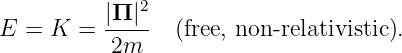 | (14.1) |
(Note that we have ignored the contribution of the rest energy to the total energy here.) In the non-relativistic case, the momentum is Π = mv, where v is the particle velocity.
If the particle is not free, but is subject to forces associated with a potential energy U(x,y,z), then equation (14.1) must be modified to account for the contribution of U to the total energy:
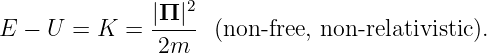 | (14.2) |
The force on the particle is related to the potential energy by
 | (14.3) |
For a free, relativistic particle, we have
 | (14.4) |
The obvious way to add forces to the relativistic case is by rewriting equation (14.4) with a potential energy, in analogy with equation (14.2):
 | (14.5) |
Unfortunately, equation (14.5) is incomplete, because we have subtracted U from the energy E without subtracting a corresponding term from the momentum Π as well. However, Π = (Π,E∕c) is a four-vector, so an equation with something subtracted from just one of the components of this four-vector is not relativistically invariant. In other words, equation (14.5) doesn’t obey the principle of relativity, and therefore cannot be correct!
How can we fix this problem? One way is to define a new four-vector with U∕c being its timelike part and some new vector Q being its spacelike part:
 | (14.6) |
We then subtract Q from the momentum Π. When we do this, equation (14.5) becomes
 | (14.7) |
The quantity Q is called the potential momentum and Q is the potential four-momentum.
Some additional terminology is useful. We define
 | (14.8) |
as the kinetic momentum for reasons discussed below. In order to avoid confusion, we rename Π the total momentum.1 Thus, the total momentum equals the kinetic plus the potential momentum, in analogy with energy.
So far, we have shown that the introduction of a potential momentum complements the potential energy so as to make the energy-momentum relationship for a particle relativistically invariant. However, we as yet have no idea what causes potential momentum nor what it does to the affected particle. We shall put off answering the former question and address only the latter at this point. A hint comes from the corresponding behavior of energy. The total energy of a particle is related to the quantum mechanical frequency ω of the particle, and the total momentum is related to its wave vector k:
 | (14.9) |
However, the kinetic energy2 and the kinetic momentum are related to the particle’s velocity v:
 | (14.10) |
where v = |v|.
The relationship between kinetic momentum and velocity can be proven by dividing equation (14.7) by ℏ to obtain a dispersion relation and then computing the group velocity, which we equate to the particle velocity. However, we will not do this here.
____________________________
Let us now study a phenomenon that depends on the existence of potential momentum. If the potential energy of a particle is zero and both the kinetic and potential momenta point in the ±x direction, the total energy equation (14.7) for the particle becomes
![E = [(Π - Q )2c2 + m2c4 ]1∕2 = (p2c2 + m2c4 )1∕2.](book230x.png) | (14.11) |
Since its total energy E is conserved, the magnitude of the kinetic momentum p of the particle doesn’t change according to the above equation. Thus, if a region of non-zero potential momentum is encountered, the total momentum of the particle must change so as to keep the kinetic momentum constant. This results in a change in the wavelength of the matter wave associated with the particle. In particular, if the potential momentum points in the same direction as the kinetic momentum, the total momentum is increased and the wavelength decreases, while a potential momentum pointing in the direction opposite the kinetic momentum results in an increase in wavelength.
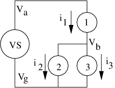
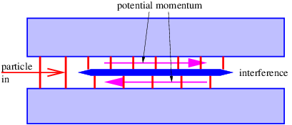
Figure 14.1 illustrates what might happen to a particle moving through a channel that splits into two sub-channels for an interval. If we arrange to have non-zero potential momenta pointing in opposite directions in the sub-channels, the wavelength of the particle will be different in the two regions. At the end of the interval, the waves recombine, interfering constructively or destructively, depending on the magnitude of the phase difference between them. If destructive interference occurs, then the particle cannot pass. The potential momentum thus acts as a valve controlling the flow of particles through the channel. This is an example of the Aharonov-Bohm effect.
In the Aharonov-Bohm effect, the potential momentum didn’t result in any force on the particle — its only manifestation was to change the particle’s wavelength. In such situations the potential momentum’s presence is only revealed by quantum mechanical effects.
The potential momentum has more of an influence on the non-quantum world when the problem is two or three-dimensional or when the potential momentum is changing with time. The total force on a particle due to all possible effects involving the potential energy and the potential momentum is given by
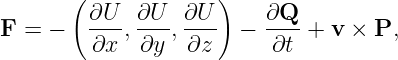 | (14.12) |
where v is the particle velocity and P is a vector obtained from the potential momentum vector as follows:
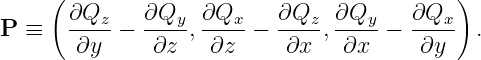 | (14.13) |
This is unexpectedly complicated. However, equation (14.12) consists of three parts. The first part involves derivatives of the potential energy and is exactly the same as in the non-relativistic case. The new effects are confined to the second and third parts, -∂Q∕∂t and v × P. A full derivation of these equations involves rather complex mathematics. However, it is possible to understand the origin of these additional contributions to the force by looking at a couple of simple examples.
A matter wave impingent on a discontinuity in potential momentum is refracted, just as it is refracted by a discontinuity in potential energy. Refraction of a matter wave packet means that the velocity of the associated particle changes as it moves across the interface. This means that the particle undergoes an acceleration, implying that it is subject to a force.
As in the case of Snell’s law for optics, the frequency of a matter wave doesn’t change as it crosses such a discontinuity in potential momentum. Furthermore, neither does the component of the wave vector parallel to the discontinuity. These two conditions together ensure phase continuity at the interface.
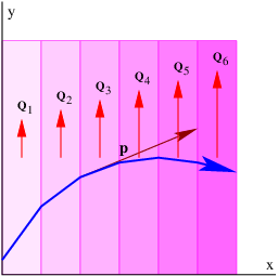
____________________________
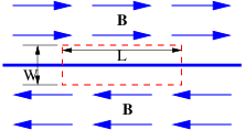
Figure 14.2 shows an example of what happens when a wave encounters a series of parallel slabs with increasing values of Q. The y component of the wave vector doesn’t change as the wave crosses each of the interfaces between slabs, for reasons discussed above. Hence, Πy = ℏky doesn’t change either, which means that dΠy∕dx = 0. The y component of kinetic momentum, py = Πy - Qy, must therefore decrease as Qy increases, as illustrated in figure 14.2.
![]()
____________________________
Newton’s second law tells us that the y component of the force on the particle associated with the wave is just the time derivative of the y component of the kinetic momentum:
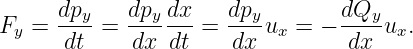 | (14.14) |
In the last step of this equation we used the fact that dΠy∕dx = 0.
The x component of the force can be obtained by similar reasoning, using the additional information that the speed, and hence the magnitude of the kinetic momentum, p2 = p x2 + p y2, doesn’t change under the influence of the potential momentum:
 | (14.15) |
Aside from assuming that p2 = constant, we have used the relationships px = (p2 - p y2)1∕2 and p y∕px = uy∕ux. Equations (14.14) and (14.15) constitute a special case of equations (14.12) and (14.13) which is valid when Q points in the y direction and is a function only of x.
The necessity for the term -∂Q∕∂t in equation (14.12) is easily understood from the following argument, which is illustrated in figure 14.3. The example in the previous section showed that a particle moving in the +x direction with velocity ux through a field of increasing Qy (left panel of figure 14.3) experiences a force in the -y direction equal to Fy = -(dQy∕dx)ux. However, viewing this same process from a reference frame in which the particle is stationary (right panel of this figure), we see that the potential momentum at the position of the particle increases with time at the rate dQy∕dt. The particle is not moving in this reference frame, so the term v×P = 0. However, the stationary particle must still experience the above force in this reference frame in order to satisfy the principle of relativity.
Noting that dQy∕dt = (dQy∕dx)ux, we see that equation (14.12) provides this force via the term -∂Q∕∂t in the reference frame moving with the particle. Thus, the time derivative term in equation (14.12) is needed to maintain the principle of relativity; the same force occurs in the two different reference frames but originates from the term v × P in the original reference frame and the term -∂Q∕∂t in the frame moving with the particle.
Arguments similar to these were actually made by Einstein in his original 1905 paper on relativity.
It turns out that the four components of the potential four-momentum are not independent, but are subject to the condition
 | (14.16) |
This is called the Lorenz condition. The physical meaning of this condition will become clear when we study electromagnetism.3
The theory of potential momentum is only one of three ways in which the idea of potential energy can be extended to the relativistic case. This theory is called gauge theory for obscure historical reasons. Gauge theory is important because electromagnetism as well as the theories of weak and strong sub-nuclear interactions are all of this type.
____________________________
Gravity is the only fundamental force that does not take the form of a gauge theory. Instead, gravity takes the form of one of two other possible relativistic extensions of potential energy. This theory is called general relativity. The gravitational force in general relativity can be interpreted geometrically as a consequence of the curvature of spacetime. Mathematically, it is far too difficult to pursue here.
The third relativistic extension of potential energy considers potential energy to be a field which alters the rest energy of particles. High energy physicists believe that the elementary particles gain their mass by this mechanism. The field is called the Higgs field after the English physicist who first proposed this theory, Peter Higgs. The recent discovery of the Higgs boson at CERN’s Large Hadron Collider in Geneva, Switzerland supports this idea.
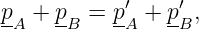
We earlier introduced the ideas of energy and momentum conservation. In other words, if we have a number of particles isolated from the rest of the universe, each with momentum pi and energy Ei, then particles may be created and destroyed and they may collide with each other.4 In these interactions the energy and momentum of each particle may change, but the sum total of all the energy and the sum total of all the momentum remains constant with time:
 | (14.17) |
The expression is simpler in terms of four-momentum:
 | (14.18) |
At this point a statement such as the one above should ring alarm bells. Just what does it mean to say that the total energy and momentum remain constant with time in the context of relativity? Which time? The time in which reference frame?
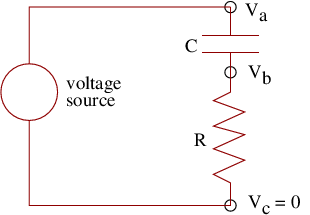
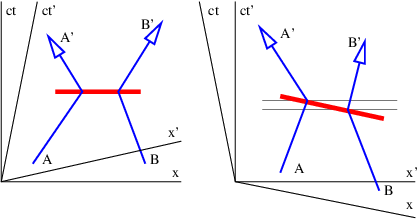
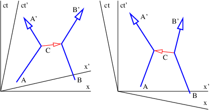
Figure 14.4 illustrates the problem. Suppose two particles exchange four-momentum remotely at the time indicated by the fat horizontal bar in the left panel of figure 14.4. Conservation of four-momentum implies that
 | (14.19) |
where the subscripted letters correspond to the particle labels in figure 14.4. Primed values refer to the momentum after the exchange while no primes indicates values before the exchange.
Now view the exchange from the reference frame in the right panel of figure 14.4. A problem with four-momentum conservation exists in the region between the thin horizontal lines. In this region particle B has already transferred its four-momentum, but it has yet to be received by particle A. In other words, four-momentum is not conserved in this reference frame!
____________________________
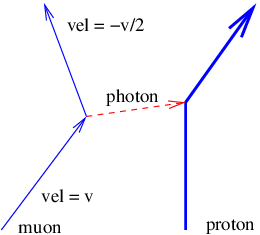
This problem is so serious that we must eliminate the concept of force at a distance from the repertoire of physics. The only way to have particles interact remotely and still conserve four-momentum in all reference frames is to assume that all remote interactions are mediated by another particle, as indicated in figure 14.5. In other words, momentum and energy are transferred from particle A to particle B in a two step process. First, particle A emits particle C in a manner which conserves the four-momentum. Second, particle C is absorbed by particle B in a similarly conservative interaction. Four-momentum is conserved at all times in all reference frames in this picture.
Another problem is evident from figure 14.5. As drawn, the velocity of the intermediary particle exceeds the speed of light. This is reflected in the fact that different reference frames yield contradictory results as to whether the intermediary particle moves from A to B or B to A. These difficulties turn out to be much less severe than those arising from non-locality. Let us address them in sequence.
For sake of definiteness, let us view the emission of particle C by particle A in a reference frame in which the velocity of particle A is just reversed in the emission process. In this case the four-momentum before the emission is pA = (p,E∕c), where E = (p2c2 + m2c4)1∕2. After the emission we have p′A = (-p,E∕c). Conservation of four-momentum in the emission process requires that
 | (14.20) |
where q is the four-momentum of particle C. From the above assumptions it is clear that
 | (14.21) |
Suppose that the real, measured mass of particle C is mC. This conflicts with the apparent or virtual mass of this particle in its flight from A to B, which is
 | (14.22) |
where q ≡|q| is the momentum transfer. Note that the apparent mass is imaginary because the four-momentum is spacelike.
Classically, this discrepancy in the apparent and actual masses of the particle C would simply indicate that the process wasn’t possible. However, recall that the uncertainty principle allows there to be an uncertainty in the mass if it doesn’t persist for too long in terms of the proper time interval along the particle’s world line. The statement of this law is ΔμΔτ ≈ 1. Expressed in terms of mass, this becomes
 | (14.23) |
Let us convert the proper time to an interval since the world line of particle C is horizontal in the reference frame in which we are viewing it. Ignoring the factor of i, Δτ = ΔI∕c. We finally compute the absolute value of the mass discrepancy as follows: |mC -iq∕c| = [(mC -iq∕c)(mC + iq∕c)]1∕2 = (m C2 + q2∕c2)1∕2. Solving for I yields the approximate maximum invariant interval that particle C can move from its source point while keeping its erroneous mass hidden by the uncertainty principle:
 | (14.24) |
A particle forced into having an apparent mass different from its actual mass is called a virtual particle. The interaction shown in figure 14.5 can only take place if particles A and B come closer to each other than the distance ΔI. This argument thus produces an estimate for the “range” of an interaction with momentum transfer 2p and intermediary particle mass mC.
Two distinct possibilities exist. If the intermediary particle is massless (a photon, for instance), then the range of the interaction is inversely related to the momentum transfer: ΔI ≈ℏ∕q. Thus, small momentum transfers can occur at large distances. An interaction of this type is called “long range”. On the other hand, if the intermediary particle has mass, the range is simply ΔI ≈ℏ∕mCc when q ≪ mCc. The range is thus constant and inversely proportional to the mass of the intermediary particle for low momentum transfers. For large momentum transfer, i. e., when q ≫ mCc, the range decreases from this value with increasing momentum transfer, as in the case of a massless intermediary particle.
According to quantum mechanics, particles are represented by waves. The absolute square of the wave amplitude represents the probability of finding the particle. In gauge theory the potential four-momentum performs this role for the virtual particles intermediary interactions. Thus a larger potential four-momentum at some point means a higher probability of finding the related virtual particles at that point.
Figure 14.5 illustrates another oddity in the role of intermediary particles in collisions. In the unprimed frame, particle C appears to be emitted by particle A and absorbed by particle B. In the primed frame the reverse is true; it appears to be emitted by B and absorbed by A. These judgements are based on the fact that the A vertex occurs earlier than the B vertex in the unprimed frame, while the B vertex occurs earlier in the primed frame. However, since these distinctions are based on time ordering in different reference frames of events separated by a spacelike interval, they are inherently not relativistically invariant. Since the principle of relativity states that physical laws are the same in all inertial reference frames, we have a conceptual problem to overcome.
A related problem has to do with the computation of energy from mass and momentum. The solution of equation E2 = p2c2 + m2c4 for the energy has a sign ambiguity that we have so far ignored:
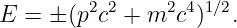 | (14.25) |
A natural tendency would be to omit the minus sign and just consider positive energies. However, this would be a mistake — experience with quantum mechanics indicates that both solutions must be considered.
Richard Feynman won the Nobel Prize in physics largely for developing a consistent interpretation of the above negative energy solutions, which we now relate. Notice that the four-momentum points backward in time in a spacetime diagram if the energy is negative. Feynman suggested that a particle with four-momentum p is equivalent to the corresponding antiparticle with four-momentum -p. Thus, we interpret a particle with momentum p and energy E < 0 as an antiparticle with momentum -p and energy -E > 0.
Antiparticles are known to exist for all particles. If a particle and its antiparticle meet, they can annihilate, creating one or more other particles. Correspondingly, if energy is provided in the right form, a particle-antiparticle pair can be created.
____________________________
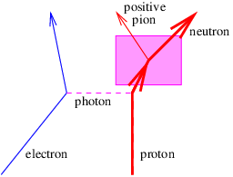
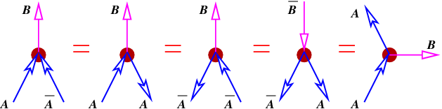
Suppose a particular kind of particle, call it an A particle, produces a B particle when it annihilates with its antiparticle A. This is illustrated in the left panel in figure 14.6. In Feynman’s view, this process is equivalent to the scattering of an A particle backward in time by a B particle, the scattering of an A backward in time by a B particle, the creation of an AA pair moving backward in time by a B particle (an antiB), and the emission of a B particle by an A particle moving forward in time.
The statement “moving backward in time” has stimulated generations of physics students to contemplate the possibility that Feynman’s picture makes time travel possible. As far as we know, this is not so. The key phrase is equivalent to. In other words, causality still works forward in time as we have come to expect.
The real utility of the “backward in time” picture is that it makes calculations easier, since processes which are normally thought of as being very different turn out to have the same mathematical form.
Returning to the ambiguity shown in figure 14.5, it turns out that it does not matter whether the picture in the left or right panel is chosen. According to the Feynman view the two processes are equivalent if one small correction is made — if the intermediary particle going from left to right is a C particle, then the intermediary particle going from right to left in the other picture is a C particle, or an antiC. It is immaterial whether the arrow representing either the C or the C points forward or backward in time. The key point is that if an arrow points into a vertex, the four-momentum of that particle contributes to the input side of the momentum-energy budget for that vertex. If an arrow points away from a vertex, then the four-momentum contributes to the output side.
If |H|≪ m and p2 ≪ m2c2, show how this equation may be approximated as
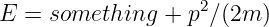
and determine the form of “something” in terms of H. Is this theory distinguishable from the theory involving potential energy at nonrelativistic velocities?
_____________________________________
_____________________________________
_____________________________________
Compute the group velocity of such a particle. Convert the result into an expression in terms of momentum rather than wavenumber. Compare this to the corresponding expression for a positive energy particle and relate it to Feynman’s explanation of negative energy states.
where q is the charge on the particle and ±mc2 is the rest energy, with the ± corresponding to positive and negative energy states. Assume that |qϕ|≪ mc2.
Hint: Recall that the total energy is always rest energy plus kinetic energy (zero in this case) plus potential energy.
In this chapter we begin the study of electromagnetism. The forces on charged particles due to electromagnetic fields are introduced and related to the general case of force on a particle by a gauge field. The principles of electric motors and generators are then addressed as an example of such forces in action.
Electromagnetism is a gauge theory. Particles that have a property called electric charge are subject to forces exerted by the gauge fields of electromagnetism. The potential four-momentum Q = (Q,U∕c) of a particle with charge q in the presence of the electromagnetic four-potential a is just
 | (15.1) |
In the simplest case the four-potential represents the amplitude for finding the intermediary particle associated with the electromagnetic gauge field. This particle has zero mass and is called the photon. If more than one photon is present, the interpretation of a becomes more complicated. This issue will be considered later.
The four-potential has space and time components A and ϕ∕c such that a = (A,ϕ∕c). The quantity A is called the vector potential and ϕ is called the scalar potential. The scalar and vector potential are related to the potential energy U and potential momentum Q of a particle of charge q by
 | (15.2) |
The Lorenz condition written in terms of A and ϕ is
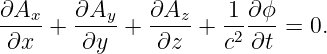 | (15.3) |
Electric and magnetic fields manifest themselves observationally by the forces that they cause. These vector quantities are related to the scalar and vector potentials as follows:
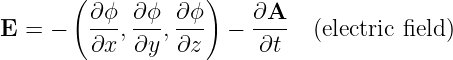 | (15.4) |
 | (15.5) |
Note that arbitrary scalar and vector constants may be added respectively to ϕ and A without changing either the electric or magnetic fields, since the latter are functions only of space and time derivatives of the former. This is a simple example of the concept of gauge invariance in action. We will see later that not just a constant, but any time-independent vector function A′(x,y,z) may be added to A with similar null results, as long as ∂Ax′∕∂y = ∂Ay′∕∂x, etc. Gauge invariance is an important part of gauge theory, but a full understanding depends on more sophisticated mathematics than currently at our disposal.
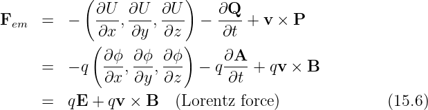
By comparison of equations (15.4) and (15.5) with the general expression for force in gauge theory, we find that the electromagnetic force on a particle with charge q is
where v is the velocity of the particle and where we have used equations (15.2) and (15.4). For historical reasons this is called the Lorentz force.
We now explore some examples of the motion of charged particles under the influence of electric and magnetic fields.
Suppose a particle with charge q is exposed to a constant electric field Ex in the x direction. The x component of the force on the particle is thus Fx = qEx. From Newton’s second law the acceleration in the x direction is therefore ax = Fx∕m = qEx∕m where m is the mass of the particle. The behavior of the particle is the same as if it were exposed to a constant gravitational field equal to qEx∕m.
If ∂A∕∂t = 0, then the electric force on a charged particle is
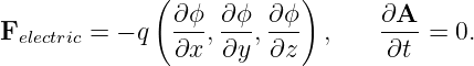 | (15.7) |
This force is conservative, with potential energy U = qϕ. Recalling that the total energy, E = K + U, of a particle under the influence of a conservative force remains constant with time, we can infer that the change in the kinetic energy with position of the particle is just minus the change in the potential energy: ΔK = -ΔU. Notice in particular that if the particle returns to its initial position, the change in the potential energy is zero and the kinetic energy recovers its initial value.
If ∂A∕∂t≠0, then there is the possibility that the electric force is not conservative. Recall that the magnetic field is derived from A. Interestingly, a necessary and sufficient criterion for a non-conservative electric force is that the magnetic field be changing with time. This result was first inferred experimentally by the English physicist Michael Faraday in 1831 and at nearly the same time by the American physicist Joseph Henry. It will be further explored later in this chapter.
____________________________
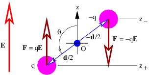
Let us now imagine a “dumbbell” consisting of positive and negative charges of equal magnitude q separated by a distance d, as shown in figure 15.1. If there is a uniform electric field E, the positive charge experiences a force qE, while the negative charge experiences a force -qE. The net force on the dumbbell is thus zero.
The torque acting on the dumbbell is not zero. The total torque acting about the origin in figure 15.1 is the sum of the torques acting on the two charges:
 | (15.8) |
The vector d can be thought of as having a length equal to the distance between the two charges and a direction going from the negative to the positive charge.
The quantity p = qd is called the electric dipole moment. (Don’t confuse it with the momentum!) The torque is just
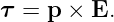 | (15.9) |
This shows that the torque depends on the dipole moment, or the product of the charge and the separation. Thus, halving the separation and doubling the charge results in the same dipole moment.
The tendency of the torque is to rotate the dipole so that the dipole moment p is parallel to the electric field E. The magnitude of the torque is given by
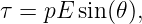 | (15.10) |
where the angle θ is defined in figure 15.1 and p = |p| is the magnitude of the electric dipole moment.
The potential energy of the dipole is computed as follows: The scalar potential associated with the electric field is ϕ = -Ez where E is the magnitude of the field, assumed to point in the +z direction. Thus, the potential energy of a single particle with charge q is U = qϕ = -qEz. The total potential energy of the dipole is the sum of the potential energies of the individual charges:
where z+ and z- are the z positions of the positive and negative charges. The equating of z+ - z- to d cos(θ) may be verified by examining the geometry of figure 15.1.The tendency of the electric field to align the dipole moment with itself is confirmed by the potential energy formula. The potential energy is lowest when the dipole moment is aligned with the field and highest when the two are anti-aligned.
____________________________
The magnetic force on a particle with charge q moving with velocity v is Fmagnetic = qv × B, where B is the magnetic field. The magnetic force is directed perpendicular to both the magnetic field and the particle’s velocity. Because of the latter point, no work is done on the particle by the magnetic field. Thus, by itself the magnetic force cannot change the magnitude of the particle’s velocity, though it can change its direction.
If the magnetic field is constant, the magnitude of the magnetic force on the particle is also constant and has the value Fmagnetic = qvB sin(θ) where v = |v|, B = |B|, and θ is the angle between v and B. If the initial velocity is perpendicular to the magnetic field, then sin(θ) = 1 and the force is just Fmagnetic = qvB. The particle simply moves in a circle with the magnetic force directed toward the center of the circle. This force divided by the mass m must equal the particle’s centripetal acceleration: v2∕R = a = F magnetic∕m = qvB∕m in the non-relativistic case, where R is the radius of the circle. Solving for R yields
 | (15.12) |
The angular frequency of revolution is
 | (15.13) |
Notice that this frequency is a constant independent of the radius of the particle’s orbit or its velocity. This is called the cyclotron frequency.
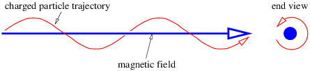
If the initial velocity is not perpendicular to the magnetic field, then the particle still has a circular component of motion in the plane normal to the field, but also drifts at constant speed in the direction of the field. The net result is a spiral motion in the direction of the magnetic field, as illustrated in figure 15.2. The radius of the circle is R = mvp∕(qB) in this case, where vp is the component of v perpendicular to the magnetic field.
____________________________
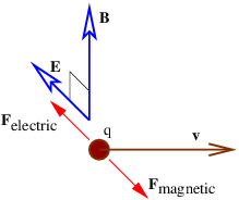
If we have perpendicular electric and magnetic fields as shown in figure 15.3, then it is possible for a charged particle to move such that the electric and magnetic forces simply cancel each other out. From the Lorentz force equation (15.6), the condition for this happening is E + v × B = 0. If E and B are perpendicular, then this equation requires v to point in the direction of E × B (i. e., normal to both vectors) with the magnitude v = |E|∕|B|. This, of course, is not the only possible motion under these circumstances, just the simplest.
It is interesting to consider this situation from the point of view of a reference frame that is moving with the charged particle. In this reference frame the particle is stationary and therefore not subject to the magnetic force. Since the particle is not accelerating, the net force, which in this frame consists only of the electric force, is zero. Hence, the electric field must be zero in the moving reference frame.
____________________________
This argument shows that the electric field perceived in one reference frame is not necessarily the same as the electric field perceived in another frame. Figure 15.4 shows why this is so. The left panel shows the situation in the reference frame moving to the right, which is the unprimed frame in this picture. The charged particle is stationary in this reference frame. The four-potential is purely spacelike, having no time component ϕ∕c. Assuming that a is constant in time, there is no electric field, and hence no electric force. Since the particle is stationary in this frame, there is also no magnetic force. However, in the primed reference frame, which is moving to the left relative to the unprimed frame and therefore is equivalent to the original reference frame in which the particle is moving to the right, the four-potential has a time component, which means that a scalar potential and hence an electric field is present.
So far we have talked mainly about point charges moving in free space. However, many practical applications of electromagnetism have charges moving through a conductor such as copper. A conductor is a material in which electrically charged particles can freely move. An insulator is a material in which charged particles are fixed in place. Practical conductors are often surrounded by insulators in order to confine the motion of charge to particular paths.
The current through a wire is defined as the amount of charge passing through the wire per unit time. When defining current, one needs to decide which direction constitutes a positive current for the problem at hand, i. e., the direction in which the positive charge is moving. If the current consists of particles carrying negative charge, then the direction of the current is opposite the direction of the motion of the particles.
Metals tend to be good conductors, while glass, plastic, and other non-metallic materials are usually insulators. All materials contain both positive and negative charges. In metals, negatively charged electrons can escape from atoms and are free to move about the material. When atoms lose one or more electrons, they become positively charged. Atoms tend to be fixed in place. Since the electron charge is negative, the current in a wire actually has a direction opposite the direction of motion of the electrons, as noted above.
____________________________
If a conductor is in the form of a wire, we can compute the magnetic force on the wire if we know the number of mobile particles per unit length of wire N, the charge on each particle q, and the speed v with which they are moving down the wire. The total force on a length of wire L is F = qNLvn × B, where n is a unit vector pointing in the direction of motion of the particles through the wire. The quantity i ≡ qNv is called the current in the wire. It equals the amount of charge per unit time flowing down the wire. Written in terms of the current, the force on a length L of the wire is
 | (15.14) |
____________________________
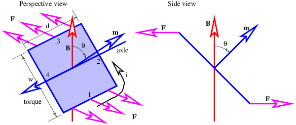
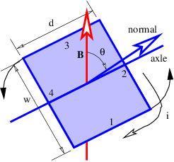
Figure 15.6 shows a rectangular loop of wire mounted on an axle in a magnetic field. A current i exists in the loop as shown. The currents in loop segments 2 and 4 experience a force parallel to the axle. These forces generate no net torque. However, the magnetic forces on loop segments 1 and 3 are each F = idB in magnitude, where B = |B| is the magnitude of the magnetic field. Together these forces generate a counterclockwise torque about the axle equal to τ = 2F(w∕2) sin(θ) = iwdB sin(θ). This can be represented in vector form as
 | (15.15) |
where m is a vector with magnitude iwd and direction normal to the loop as shown in figure 15.6. The vector m is called the magnetic dipole moment.
The loop can actually be any shape, not just rectangular. In the general case the magnitude of the magnetic moment equals the current i times the area S of the loop:
 | (15.16) |
In the above example the area is S = wd. The direction of m is determined by the right hand rule; curl the fingers on your right hand around the loop in the direction of the current and your thumb points in the direction of m.
In analogy with the electric dipole in an electric field, the potential energy of a magnetic dipole in a magnetic field is
 | (15.17) |
Figure 15.6 illustrates the principle of an electric motor. A motor consists of multiple loops of wire on an axle carrying a current in a magnetic field. The torque on the axle turns the loops so that the magnetic moment is parallel to the field. The angular momentum of the loops carries the rotation of the axle through the zero torque region, which occurs when the magnetic moment is either perfectly parallel or perfectly anti-parallel (i. e., pointing in the opposite direction) to the field. At this point either the magnetic field is reversed by some mechanism or the magnetic dipole is reversed by making the current circulate around the loops in the opposite direction. The torque due to the magnetic force then turns the axle through another half-turn, whereupon the field or the magnetic moment is again reversed, and so on.
As was shown earlier, the electric field is derived from two different sources, spatial derivatives of the scalar potential and time derivatives of the vector potential:
 | (15.18) |
In time independent situations the vector potential part drops out and we are left with a dependence only on the scalar potential. In this case a particle with charge q has an electrostatic potential energy U = qϕ, which means that the electric force is conservative. However, in the time dependent situation there is no guarantee that the part of the electric field derived from the vector potential will be conservative.
____________________________
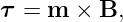
An example of a non-conservative electric field occurs when we have
 | (15.19) |
where C is a constant. In this case the electric and magnetic fields are
 | (15.20) |
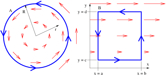
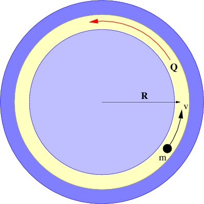
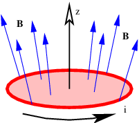
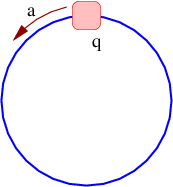
The magnetic field points in the -z direction and increases in magnitude with time. The electric field vectors are shown in figure 15.7. Notice that a positively charged particle moving in a counterclockwise circle as shown is continually being accelerated in the direction of motion, and is therefore continually gaining energy. This is impossible with a conservative force.
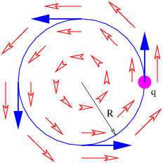
How much energy is gained by a particle with charge q moving in a complete circle of radius R under the above circumstances? The magnitude of the electric field at this radius is E = CR, so the force on the particle is F = qCR. The circumference of the circle is 2πR, so the total work done by the electric field in one revolution is just ΔW = 2πRF = 2πqCR2 = 2qCS, where S = πR2 is the area of the circle. Let us define ΔV = ΔW∕q = 2CS. For historical reasons this is called the electromotive force or EMF. This is deceptive terminology, because in fact ΔV doesn’t have the dimensions of force — it is really just the work per unit charge done on a particle making a single loop around the circle in figure 15.7.
Recall that the z component of the magnetic field in this case is Bz = -2Ct. Note that the time derivative of the magnetic field is just ∂Bz∕∂t = -2C. Comparison with the equation for electromotive force shows us that
 | (15.21) |
where the area is brought inside the time derivative since it is constant in time.
____________________________
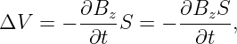
Notice that the argument of the time derivative in the above equation is the component of B perpendicular to the plane of the loop. The loop area multiplied by the normal component of B is the magnetic flux through the loop: ΦB ≡ BnormalS. The generalization of equation (15.21) for any loop fixed in space is expressed as
 | (15.22) |
It is valid for arbitrary loop and magnetic field configurations, not just for the simple case we have been investigating.
The minus sign in equation (15.22) means the following: If the fingers on your right hand curl around the loop in the direction opposite to the direction that causes a positive charge to gain energy, then your thumb points in the direction of the time rate of change of the magnetic flux passing through the loop. This is illustrated in figure 15.8.
If a loop is changing size or shape with time, then the magnetic force also acts on charges in the loop. The work per unit charge done in a segment j of the loop defined by the displacement vector Δlj is
 | (15.23) |
where vj is the velocity with which the loop segment is moving and Bj is the magnetic field at the location of the segment. To get the total EMF around the loop due to the magnetic force, the ΔV j values from each segment must simply be summed up and added to the right side of equation (15.22):
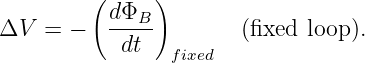
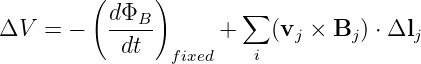 | (15.24) |
It turns out that the part of ΔV resulting from a moving or deforming loop equals minus the time rate of change of magnetic flux through the loop due solely to loop movement and deformation. Therefore, we can rewrite equation (15.24) in the more compact form
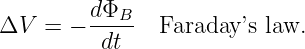 | (15.25) |
where the time derivative of the magnetic flux now includes both changes in the magnetic field and changes in the position, shape, and orientation of the loop. This is called Faraday’s law, even though it is a hybrid of equation (15.22), which is Faraday’s law as generally defined in advanced physics and the Lorentz force law as expressed in equation (15.23).
____________________________
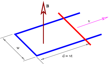
The electric generator is perhaps the best known application of Faraday’s law. Figure 15.9 shows a rectangular loop of wire fixed to an axle that rotates at an angular rate Ω. The magnetic flux through the loop thus varies with time according to ΦB = wdB cos(θ) = wdB cos(Ωt). The EMF around the loop is thus
 | (15.26) |
In a real generator there are many loops forming a coil of wire and the ends of the coil are brought out through the axle so that the resulting current can be tapped for practical use.
The EMF ΔV has the same units as the scalar potential ϕ. What is the difference between the two quantities? Both are related to the work done per unit charge by the electric field on a particle moving through the field. However, recall that the electric field is composed of two parts:
 | (15.27) |
Δϕ = ϕ2 - ϕ1 is minus the work done on the particle in going from point 1 to point 2 by the part of the electric field associated with the scalar potential; moving to a lower potential results in a release of kinetic energy according to the conservation of energy. On the other hand, ΔV is (plus) the work done per unit charge on a particle by the part of the electric field associated with the time derivative of the vector potential.
Aside from the different sign conventions, there is one other fundamental difference between the two quantities: Δϕ is always zero for closed paths, i. e., paths in which the particle returns to its initial point. This is because point 1 is then the same as point 2, so ϕ1 = ϕ2. This condition doesn’t necessarily apply to the EMF. ΔV often is non-zero for closed particle paths. The electric generator that we have just discussed is an important case in point. The total work done per unit charge by the electric field on a charged particle moving along some path is thus ΔV - Δϕ. The Δϕ term drops out if the path is closed.
_____________________________________
_____________________________________
_____________________________________
_____________________________________
In this chapter we investigate how charge produces electric and magnetic fields. We first introduce Coulomb’s law, which is the basis for everything else in the section. We then discuss Gauss’s law for the electric and magnetic field, drawing on what we learned while using it on the gravitational field. Coulomb’s law and the theory of relativity together show that magnetic fields are generated by moving charge. We then use this fact to compute the magnetic fields from some simple charge distributions. We finish with a discussion of electromagnetic waves.
A stationary point electric charge q is known to produce a scalar potential
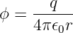 | (16.1) |
a distance r from the charge. The constant ϵ0 = 8.85 × 10⁻¹² C2 N-1 m-2 is called the permittivity of free space. The vector potential produced by a stationary charge is zero.
The potential energy between two stationary charges is equal to the scalar potential produced by one charge multiplied by the value of the other charge:
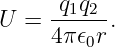 | (16.2) |
Notice that it doesn’t make any difference whether one multiplies the scalar potential from charge 1 by charge 2 or vice versa – the result is the same.
Since r = (x2 + y2 + z2)1∕2, the electric field produced by a charge is
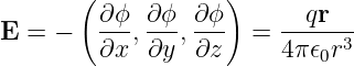 | (16.3) |
where r = (x,y,z) is the vector from the charge to the point where the electric field is being measured. The magnetic field is zero since the vector potential is zero.
The force between two stationary charges separated by a distance r is the value of one charge multiplied by the electric field produced by the other charge. Thus the magnitude of the force is
 | (16.4) |
with the force being repulsive if the charges are of the same sign, and attractive if the signs are opposite. This is called Coulomb’s law.
Equation (16.4) is the electric equivalent of Newton’s universal law of gravitation. Replacing mass by charge and G by -1∕(4πϵ0) in the equation for the gravitational force between two point masses gives us equation (16.4). The most important aspect of this result is that both the gravitational and electrostatic forces decrease as the square of the distance between the particles.
The electric flux is defined in analogy to the gravitational flux as
 | (16.5) |
where S is the directed area through which the flux passes. (This is strictly true only for small, flat areas S over which the component of E normal to S can be assumed constant.) Since the electric field obeys an inverse square law, Gauss’s law applies to the electric flux ΦE just as it applies to the gravitational flux. In particular, since the magnitude of the outward electric field a distance r from a charge q is E = q∕(4πϵ0r2), the electric flux through a sphere of radius r (and area 4πr2) concentric with the charge is ES = [q∕(4πϵ 0r2)] × (4πr2) = q∕ϵ 0. This generalizes to an arbitrary distribution of charge as in the gravitational case:
 | (16.6) |
where ΦE in this equation is the outward electric flux through a closed surface and qinside is the net charge inside this surface. This is an expression of Gauss’s law for the electric field. Since Gauss’s law for electricity and for gravitation are so similar, we can use all our insights from studying gravity on the electric field case.
____________________________
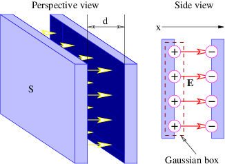
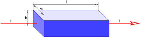
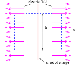
Figure 16.1 shows how to set up the Gaussian surface to obtain the electric field emanating from an infinite sheet of charge. We assume a charge density of σ Coulombs per square meter, which means that the amount of charge inside the box is qinside = σhd, where the box has height h and depth d into the page. The total electric flux out of the left and right faces of the box is ΦE = 2Ehd, where E is the magnitude of the electric field on these surfaces. The field is assumed to point away from the charge, and hence out of the box on both faces. Due to the assumed direction of the electric field, there is no electric flux out of any of the other faces of the box.
Applying Gauss’s law, we infer that 2Ehd = σhd∕ϵ0, which means that the electric field emanating from a sheet of charge with charge density per unit area σ is
 | (16.7) |
The scalar potential associated with this electric field is easily obtained by realizing that equation (16.7) gives the x component of this field — the other components are zero. Using E = -∂ϕ∕∂x, we infer that
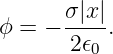 | (16.8) |
The absolute value signs around x take account of the fact that the direction of the electric field for negative x is opposite that for positive x.
____________________________
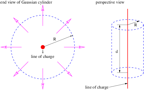
Similar reasoning is used to obtain the electric field due to a line of charge. A sketch of the expected electric field vectors and a Gaussian cylinder coaxial with the line of charge is shown in figure 16.2. If the charge per unit length is λ, the amount of charge inside the cylinder is qinside = λd, where d is the length of the cylinder. The outward electric flux at radius r is ΦE = 2πrdE. Gauss’s law therefore tells us that the electric field at radius r is just
 | (16.9) |
In this case E = -∂ϕ∕∂r, so that the scalar potential is
 | (16.10) |
____________________________
By analogy with Gauss’s law for the electric field, we could write a Gauss’s law for the magnetic field as follows:
 | (16.11) |
where ΦB is the outward magnetic flux through a closed surface, C is a constant, and qmagnetic inside is the “magnetic charge” inside the closed surface. Extensive searches have been made for magnetic charge, generally called a magnetic monopole. However, none has ever been found. Thus, Gauss’s law for magnetism can be written
 | (16.12) |
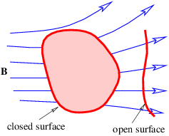
This of course doesn’t preclude non-zero values of the magnetic flux through open surfaces, as illustrated in figure 16.3.
The equation (16.1) for the scalar potential of a point charge is valid only in the reference frame in which the charge q is stationary. By symmetry, the vector potential must be zero. Since ϕ is actually the timelike component of the four-potential, we infer that the four-potential due to a charge is tangent to the world line of the charged particle.
A consequence of the above argument is that a moving charge produces a magnetic field, since the four-potential must have spacelike components in this case.
We have shown that electric charge generates both electric and magnetic fields, but the latter result only from moving charge. If we have the scalar potential due to a static configuration of charge, we can use this result to find the magnetic field if this charge is set in motion. Since the four-potential is tangent to the particle’s world line, and hence is parallel to the time axis in the reference frame in which the charged particle is stationary, we know how to resolve the space and time components of the four-potential in the reference frame in which the charge is moving.
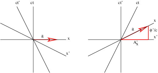
____________________________
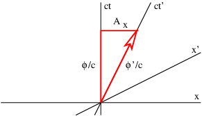
Figure 16.4 illustrates this process. For a particle moving in the +x direction at speed v, the slope of the time axis in the primed frame is just c∕v. The four-potential vector has this same slope, which means that the space and time components of the four-potential must now appear as shown in figure 16.4. If the scalar potential in the primed frame is ϕ′, then in the unprimed frame it is ϕ, and the x component of the vector potential is Ax. Using the spacetime Pythagorean theorem, ϕ′2∕c2 = ϕ2∕c2 - A x2, and relating slope of the ct′ axis to the components of the four-potential, c∕v = (ϕ∕c)∕Ax, it is possible to show that
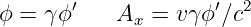 | (16.13) |
where
 | (16.14) |
Thus, the principles of special relativity allow us to obtain the full four-potential for a moving configuration of charge if the scalar potential is known for the charge when it is stationary. From this we can derive the electric and magnetic fields for the moving charge.
____________________________
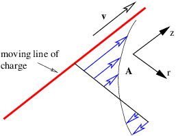
As an example of this procedure, let us see if we can determine the magnetic field from a line of charge with linear charge density in its own rest frame of λ′, aligned along the z axis. The line of charge is moving in a direction parallel to itself. From equation (16.10) we see that the scalar potential a distance r from the z axis is
 | (16.15) |
in a reference frame moving with the charge. The z component of the vector potential in the stationary frame is therefore
 | (16.16) |
by equation (16.13), with all other components being zero. This is illustrated in figure 16.5.
____________________________
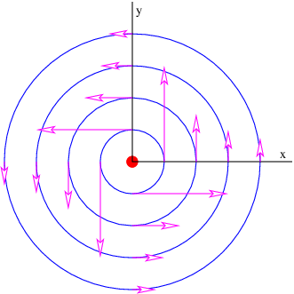
We infer that
 | (16.17) |
where we have used r2 = x2 + y2. The resulting field is illustrated in figure 16.6. The field lines circle around the line of moving charge and the magnitude of the magnetic field is
 | (16.18) |
There is an interesting relativistic effect on the charge density λ′, which is defined in the co-moving or primed reference frame. In the unprimed frame the charges are moving at speed v and therefore undergo a Lorentz contraction in the z direction. This decreases the charge spacing by a factor of γ and therefore increases the charge density as perceived in the unprimed frame to a value λ = γλ′.
We also define a new constant μ0 ≡ 1∕(ϵ0c2). This is called the permeability of free space. This constant has the assigned value μ0 = 4π × 10-7 N s2 C-2. The value of ϵ0 = 1∕(μ0c2) is actually derived from this assigned value and the measured value of the speed of light. The reasons for this particular way of dealing with the constants of electromagetism are obscure, but have to do with making it easy to relate the values of constants to the experiments used in determining them.
With the above substitutions, the magnetic field equation becomes
 | (16.19) |
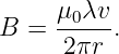
The combination λv is called the current and is symbolized by i. The current is the charge per unit time passing a point and is a fundamental quantity in electric circuits. The magnetic field written in terms of the current flowing along the z axis is
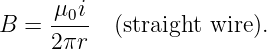 | (16.20) |
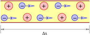
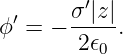
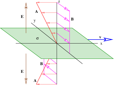
As another example we consider a uniform infinite sheet of charge in the x - y plane with charge density σ′. The charge is moving in the +x direction with speed v. As we showed in the section on Gauss’s law for electricity, the electric field for this sheet of charge in the co-moving reference frame is in the z direction and has the value
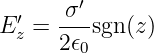 | (16.21) |
where we define
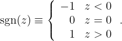 | (16.22) |
The sgn(z) function is used to indicate that the electric field points upward above the sheet of charge and downward below it (see figure 16.7).
The scalar potential in this frame is
 | (16.23) |
____________________________
In the stationary reference frame in which the sheet of charge is moving in the x direction, the scalar potential and the x component of the vector potential are
 | (16.24) |
according to equation (16.13), where σ = γσ′ is the charge density in the stationary frame. The other components of the vector potential are zero. We calculate the magnetic field as
 | (16.25) |
where sgn(z) is defined as before. The vector potential and the magnetic field are shown in figure 16.7. Note that the magnetic field points normal to the direction of motion of the charge but parallel to the sheet. It points in opposite directions on opposite sides of the sheet of charge.
We have found so far that stationary charge produces an electric field while moving charge produces a magnetic field. It turns out that accelerated charge produces electromagnetic radiation. Electromagnetic radiation is nothing more than one or more photons that have zero mass, and are therefore real, not virtual.
____________________________
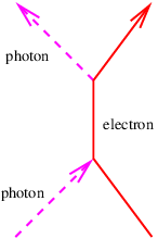
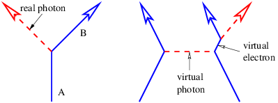
Acceleration of a charged particle is needed to produce radiation because of the conservation of energy and momentum. The left panel of figure 16.8 shows why. Since a photon carries off energy and momentum, conservation means that the energy and momentum of the emitting particle change due to the emission of a photon. This corresponds in classical mechanics to an acceleration.
The process in the left panel of figure 16.8 actually cannot occur if particles A and B have the same mass. If the mass of the outgoing particle B is less than the mass of the incoming particle A, then this reaction can and does occur. An example is the decay of an atom from a higher energy state to a lower energy state (and hence lower mass), accompanied by the emission of a photon.
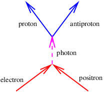
Another type of reaction that can generate radiation occurs when two charged particles (say, electrons) collide, as illustrated in the right panel of figure 16.8. In an elastic collision both electrons are real both before and after the photon transfer. However, it is possible for one of the electrons to have a virtual mass that is greater than the normal electron mass after the collision, which means that it is free to decay to a real electron plus a real photon.
We now try to understand the characteristics of free electromagnetic radiation. In our studies of waves we found it easiest to examine plane waves. We will follow this path here, writing the four-potential for an electromagnetic plane wave moving in the x direction as
 | (16.26) |
where a0 = (A0,ϕ0∕c) is a constant four-vector representing the direction and maximum amplitude of the four-potential, and kx and ω are the wavenumber and the angular frequency of the wave. Since the real photon is massless, we have ω = kxc in this case. Virtual photons are not subject to this constraint.
By substituting A and ϕ from equation (16.26) into the Lorenz condition, we find that
 | (16.27) |
Thus, the Lorenz condition requires that the scalar potential ϕ be related to the x or longitudinal component of the vector potential, Ax, i. e., the component pointing in the direction of wave propagation. The transverse components, Ay and Az, are unconstrained by the Lorenz condition, since they don’t depend on y and z.
Using equations for the electric and magnetic field, as well as equations (16.26) and (16.27), we can now find E and B in an electromagnetic plane wave:
 | (16.28) |
 | (16.29) |
The electric field has a longitudinal or x component proportional to kxϕ0 -ωA0x = -ω(ϕ0∕c-A0x). However, comparison with equation (16.27) shows that Ex = 0 as long as ω∕kx = c, i. e., as long as the photons travel at the speed of light, c. Thus, virtual photons, i. e., those that have a non-zero mass and therefore travel at a speed other than that of light, can have a non-zero longitudinal component of the electric field, but real photons cannot.
The dot product of the electric and magnetic fields in a plane wave is E ⋅ B = 0, as can be verified from equations (16.28) and (16.29). This means that E and B are perpendicular to each other. Furthermore, both E and B are perpendicular to the direction of wave motion for real photons.
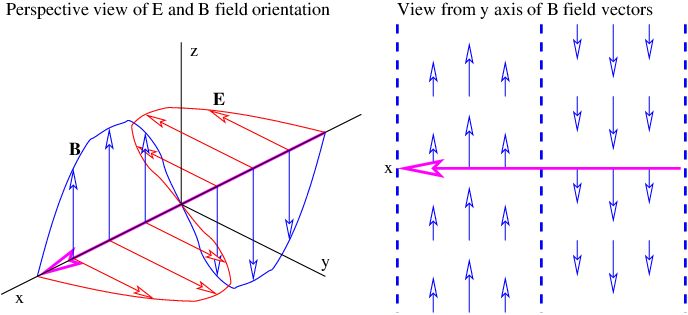
____________________________
Figure 16.9 shows the electric and magnetic fields for real photons in the special case where Az = 0. The electric field points in the same direction as the transverse part of the vector potential, while the magnetic field points in the other transverse direction. The ratio of the magnitudes of the electric and magnetic fields is easily inferred from equations (16.28) and (16.29):
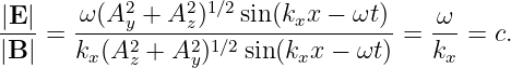 | (16.30) |
Notice that the electric and magnetic fields for a wave do not depend on the longitudinal component of the vector potential, Ax. This is because the Lorenz condition forces Ax to cancel with the term containing ϕ in the expression for Ex.
We are now in a position to see what the Lorenz condition means. For an isolated stationary charge, the scalar potential is given by equation (16.1) and the vector potential A is zero. The Lorenz condition reduces to
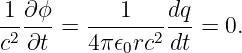 | (16.31) |
From this we see that the Lorenz condition applied to the four-potential for a point charge is equivalent to the statement that the charge on a point particle is conserved, i. e., it doesn’t change with time. This is extended to any stationary distribution of charge by the superposition principle.
We thus see that the Lorenz condition is closely related to charge conservation for the four-potential of any charge distribution in the reference frame in which the charge is stationary. If we can further show that the Lorenz condition is an equation that is equally valid in all reference frames, then we will have demonstrated that it is true for the four-potential produced by moving charged particles as well.
If the Lorenz condition is valid in one reference frame, it is valid in all frames for the special case of a plane electromagnetic wave. This follows from substituting the four-potential for a plane wave into the Lorenz condition, as was done in equation (16.27) in the previous section. In this case the Lorenz condition reduces to k ⋅ a = 0. Since the dot product of two four-vectors is a relativistic scalar, the Lorenz condition is equally valid in all frames.
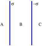
_____________________________________
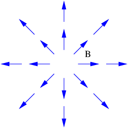
_____________________________________
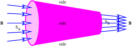
_____________________________________
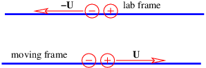
_____________________________________
Various electronic devices are considered in this chapter. This is useful not only for understanding these devices but also for revealing new aspects of electromagnetism. The capacitor is first discussed and Ampère’s law is introduced. The theory of magnetic inductance is then developed. Ohm’s law and the resistor are discussed. The energy associated with electric and magnetic fields is calculated and Kirchhoff’s laws for electric circuits are briefly discussed.
We first discuss a device that is commonly used in electronics, called the capacitor. We then introduce a new mathematical idea called the circulation of a vector field around a loop. Finally, we use this idea to investigate Ampère’s law.
The capacitor is an electronic device for storing charge. The simplest type is the parallel plate capacitor, illustrated in figure 17.1. This consists of two conducting plates of area S separated by distance d, with the plate separation being much smaller than the plate dimensions. Positive charge q resides on one plate, while negative charge -q resides on the other.
The electric field between the plates is E = σ∕ϵ0, where the charge per unit area on the inside of the left plate in figure 17.1 is σ = q∕S. The density on the right plate is just -σ. All charge is assumed to reside on the inside surfaces and thus contributes to the electric field crossing the gap between the plates.
The above formula for the electric field comes from applying Gauss’s law to the sheet of charge on the positive plate. The factor of 1∕2 present in the equation for an isolated sheet of charge is absent here because all of the electric flux exits the Gaussian surface on the right side — the left side of the Gaussian box is inside the conductor where the electric field is zero, at least in a static situation.
There is no vector potential in this case, so the electric field is related solely to the scalar potential ϕ. Integrating Ex = -∂ϕ∕∂x across the gap between the conducting plates, we find that the potential difference between the plates is Δϕ = Exd = qd∕(ϵ0S), since Ex is known to be constant in this case. This equation indicates that the potential difference Δϕ is proportional to the charge q on the left plate of the capacitor in figure 17.1. The constant of proportionality is d∕(ϵ0S), and the inverse of this constant is called the capacitance:
 | (17.1) |
The relationship between potential difference, charge, and capacitance is thus
 | (17.2) |
The equation for the capacitance of the illustrated parallel plates contains just a fundamental constant (ϵ0) and geometrical factors (area of plates, spacing between them), and represents the amount of charge the parallel plate capacitor can store per unit potential difference between the plates. A word about signs: The higher potential is always on the plate of the capacitor that has the positive charge.
Note that equation (17.1) is valid only for a parallel plate capacitor. Capacitors come in many different geometries and the formula for the capacitance of a capacitor with a different geometry will differ from this equation. However, equation (17.2) is valid for any capacitor.
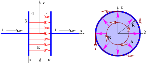
____________________________
We now show that a capacitor that is charging or discharging has a magnetic field between the plates. Figure 17.2 shows a parallel plate capacitor with a current i flowing into the left plate and out of the right plate. This current is necessarily accompanied by an electric field that is changing with time: Ex = q∕(ϵ0S) = it∕(ϵ0S). Such an electric field can be derived from a scalar potential that is a function of time: ϕ = -itx∕(ϵ0S). However, the Lorenz condition
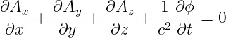 | (17.3) |
demands that some component of the vector potential A be non-zero under these circumstances, since ∂ϕ∕∂t is non-zero.
How much can we infer about the vector potential from the geometry of the capacitor and equation (17.3)? Substituting ϕ = -itx∕(ϵ0S) into this equation results in
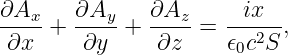 | (17.4) |
which suggests a number of different possibilities for A. For instance, A = (0,ixy∕(ϵ0c2S), 0) and A = [0, 0,ixz∕(ϵ 0c2S)] both satisfy equation (17.4). However, neither of these trial choices is satisfactory by itself, as they are not consistent with the cylindrical symmetry of the capacitor about the x axis.
A choice of vector potential that is consistent with the shape of the capacitor and satisfies the Lorenz condition is obtained by combining these two trial solutions:
![A = [0,ixy ∕(2ϵ c2S ),ixz∕(2ϵ c2S)].
0 0](book2111x.png) | (17.5) |
This vector potential leads to the magnetic field
![B = [0,- iz∕ (2ϵ0c2S ),iy∕ (2 ϵ0c2S )].](book2112x.png) | (17.6) |
These fields are illustrated in the right-hand panel of figure 17.2.
We have already seen one example of the circulation1 of a vector field, though we didn’t label it as such. In chapter 15 we computed the work done on a charge by the electric field as it moves around a closed loop in the context of the electric generator and Faraday’s law. The work done per unit charge, or the EMF, is an example of the circulation of a field, in this case the electric field, ΓE. Faraday’s law can be restated as
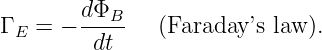 | (17.7) |
In the simple case of a circular loop with the field directed along the loop, the circulation is just the magnitude of the field multiplied by the circumference of the loop, as illustrated in the left panel of figure 17.3. In more complicated cases in which the field points in a direction other than the direction of the loop, just the component in the direction of traversal around the loop enters the circulation. If this component varies as one progresses around the loop, the calculation must be broken into pieces. The total circulation is then obtained by adding up the contributions from segments of the loop in which the value of the field component parallel to the motion around the loop is constant. An example of this type is the calculation of the EMF around a square loop of wire in an electric generator. Another is illustrated in the right panel of figure 17.3.
The magnetic circulation ΓB around the periphery of the capacitor in the right panel of figure 17.2 is easily computed by taking the magnitude of B in equation (17.6). The magnitude of the magnetic field on the inside of the capacitor is just B = ir∕(2ϵ0c2S), since r = (y2 + z2)1∕2 in figure 17.2. Thus, at the periphery of the capacitor, r = R, and B = iR∕(2ϵ0c2S) there. The area of the capacitor plates is S = πR2 and ϵ 0c2 = 1∕μ 0, as we discussed previously. Thus, the magnetic field is B = μ0i∕(2πR) at the periphery. If the periphery is traversed in the counter-clockwise direction, the magnetic circulation around the capacitor is ΓB = 2πRB = μ0i.
Let us now compute the magnetic circulation around a wire carrying a current. The magnetic field a distance r from a straight wire carrying a current i is B = μ0i∕(2πr). The magnetic field points in the direction of a circle concentric with the wire. The magnetic circulation around the wire is thus ΓB = 2πrB = μ0i.
Notice that the magnetic circulation is found to be the same around the wire and around the periphery of the capacitor. Furthermore, this circulation depends only on the current in the wire and the constant μ0.
One further item needs to be calculated, namely the electric flux across the gap between the capacitor plates. This is just the electric field E = σ∕ϵ0 multiplied by the area S, or ΦE = Sσ∕ϵ0 = q∕ϵ0. The current into the capacitor is the time rate of change on the capacitor, so i = dq∕dt = ϵ0dΦE∕dt.
We are now in a position to understand Ampère’s law:
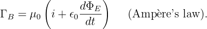 | (17.8) |
This states that the magnetic circulation around a loop equals the sum of two contributions, (1) μ0 multiplied by the electric current through the loop and (2) μ0ϵ0 multiplied by the time rate of change of the electric flux through the loop. In the above example the first term dominates when the loop is around the wire, while the second term acts when the loop is around the gap between the capacitor plates.
Ampère actually formulated an incomplete version of the law named after him — he included only the first term containing the current. The Scottish physicist James Clerk Maxwell added the second term, based primarily on theoretical reasoning. Maxwell’s additional term solved a serious internal inconsistency in electromagnetic theory — in our terms, the Lorenz condition requires a magnetic field to exist if the scalar potential ϕ is time-dependent. This magnetic field is only predicted by Ampère’s law if Maxwell’s term is included. The quantity ϵ0dΦE∕dt was called the displacement current by Maxwell since it has the dimensions of current and is numerically equal to the current entering the capacitor. However, it isn’t really a current — it is just an electric flux that changes with time!
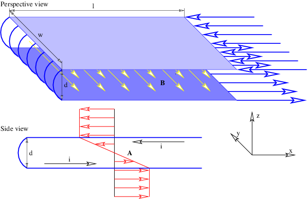
____________________________
Gauss’s law for electricity and magnetism, Faraday’s law, and Ampère’s law are collectively called Maxwell’s equations. Together they form the basis for electromagnetism as it developed historically. However, our formulation of electromagnetism in terms of the four-potential, the dispersion relation for free electromagnetic waves, the Lorenz condition, and Coulomb’s law, is precisely equivalent to Maxwell’s equations, and is much closer to the modern approach to electromagnetism.
Induction is the tendency of a current in a conductor to maintain itself in the face of changes in the potential difference driving the current. Figure 17.4 shows a parallel plate inductor in which a current i passes through the two plates in opposite directions.2 The vector potential between plates of width w and spacing d is
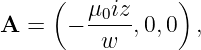 | (17.9) |
as long as w ≫ d (see figure 17.4).
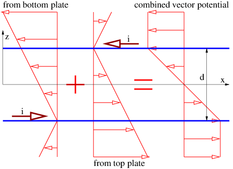
____________________________
Let us try to understand how this vector potential is constructed from what we already know. The vector potential for a single current sheet in the x-y plane at z = 0 moving in the x direction was computed in the previous chapter as Ax = -vσ|z|∕(2ϵ0c2), with A y = Az = 0. The quantity σ is the charge per unit area on the sheet and v is the velocity of the charge sheet in the x direction. We use the relationship 1∕(ϵ0c2) = μ 0 and also realize that if each plate has a width w, then the current in each plate is i = vσw, which means that we can rewrite Ax = -μ0i|z|∕(2w) for a single plate.
To proceed further, we first need to understand that |z| in the above equation is only valid if the charge sheet is at z = 0. If the sheet is located a distance a from the origin, then we must replace |z| by |z - a|. We also need to call on the definition of absolute value to realize that |z - a| = z - a if z > a, and |z - a| = -z + a if z < a. Figure 17.5 shows how the profiles of Ax from each of the charge sheets add together to form a combined profile for the two sheets together.
The resulting magnetic field between the plates can be computed from the vector potential:
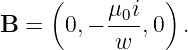 | (17.10) |
Above and below the plates the magnetic field is zero because the vector potential is constant.
Let us now ask what happens when the current through the inductor increases or decreases with time. Assuming initially that no scalar potential exists, the x component of the electric field in the device is
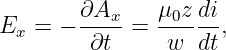 | (17.11) |
while Ey = Ez = 0. Substituting the z values for each plate, we see that
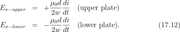
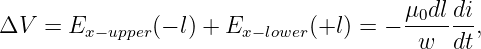 | (17.13) |
where l is the length of the plate, as illustrated in figure 17.4.
The minus sign means that the electric field acts so as to oppose a change in the current. This result is called Lenz’s law. Lenz’s law is not an independent law, but arises from the minus sign in the statement of Faraday’s law.
In order for the current i through the inductor to increase with time, an external potential difference Δϕ must be imposed between the input and output wires of the inductor, which just balances the effects of the internally generated electric field:
 | (17.14) |
If this potential difference is positive, i. e., if the input wire of the inductor is at a higher potential then the output wire, then the current through the inductor will increase with time. If it is lower, the current will decrease.
As with capacitors, inductors come in many shapes and forms. The above equation is valid only for a parallel plate inductor, but the relationship
 | (17.15) |
is valid for any inductor, assuming that the inductance L is known. Comparison of the above two equations reveals that the inductance for the parallel plate inductor shown in figure 17.4 is just
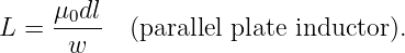 | (17.16) |
Normal conducting materials require an electric field to keep an electric current flowing through them. The electric field causes a force on the electrons in the material, which is balanced by the energy loss that occurs when the electrons collide with the atoms forming the material. Most objects exhibit a linear relationship between the current i through them and the potential difference Δϕ applied to them. This relationship is called Ohm’s law,
 | (17.17) |
where the constant of proportionality R is called the resistance. The quantity Δϕ is sometimes called the voltage drop across the resistor.
For certain materials, such as semiconductors, the resistance depends on the current. For such materials, the above equation defines resistance, but since the resistance doesn’t remain constant when the current changes, these materials don’t obey Ohm’s law.
Figure 17.6 illustrates a rectangular resistor. The resistance of such a resistor can be written
 | (17.18) |
where the resistivity ρ is characteristic only of the material and not its shape or size.
Unlike capacitors and inductors, resistors are dissipative devices. The work done on a charge q passing through a resistor is just qΔϕ. This energy is converted to heat. The work done per unit time, which equals the power dissipated by a resistor is therefore
 | (17.19) |
In this section we calculate the energy stored by a capacitor and an inductor. It is most profitable to think of the energy in these cases as being stored in the electric and magnetic fields produced respectively in the capacitor and the inductor. From these calculations we compute the energy per unit volume in electric and magnetic fields. These results turn out to be valid for any electric and magnetic fields — not just those inside parallel plate capacitors and inductors!
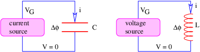
____________________________
Let us first consider a capacitor starting in a discharged state at time t = 0. A constant current i is caused to flow through the capacitor by some device such as a battery or a generator, as shown in the left panel of figure 17.7. As the capacitor charges up, the potential difference across it increases with time:
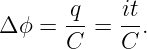 | (17.20) |
The EMF supplied by the generator has to increase to match this value.
The generator does work on the positive charges moving around the circuit in the direction indicated by the arrow. We assume that Δϕ equals the EMF or work per unit charge done by the generator V G, so the work done in time dt by the generator is dW = V Gdq = V Gidt. Using the equation for the potential difference across a capacitor, we see that the power input is
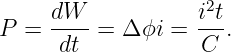 | (17.21) |
Integrating this in time yields the total energy UE supplied to the capacitor by the generator:
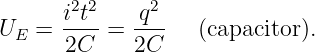 | (17.22) |
Assuming that we have a parallel plate capacitor, let’s insert the formula for the capacitance of such a device, C = ϵ0S∕d. Let us further recall that the electric field in a parallel plate capacitor is E = σ∕ϵ0 = q∕(ϵ0S), so that q = ϵ0ES and
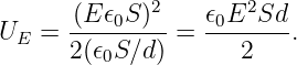 | (17.23) |
The combination Sd is just the volume between the capacitor plates. The energy density in the capacitor is therefore
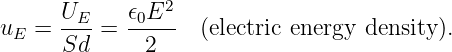 | (17.24) |
This formula for the energy density in the electric field is specific to a parallel plate capacitor. However, it turns out to be valid for any electric field.
A similar analysis of a current increasing from zero in an inductor yields the energy density in a magnetic field. Imagine that the generator in the right panel of figure 17.7 produces a constant EMF, V G, starting at time t = 0 when the current is zero. The work done by the generator in time dt is dW = V Gdq = V Gidt so that the power is
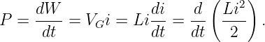 | (17.25) |
We have assumed that the EMF supplied by the generator, V G, balances the voltage drop across the inductor: V G = Δϕ = L(di∕dt).
If we integrate the above equation in time, we get the energy added to the inductor as a result of increasing the current through it. Substituting the formula for the inductance of a parallel plate inductor, L = μ0dl∕w, we arrive at the equation for the energy stored by the inductor:
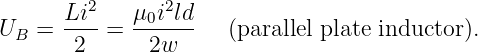 | (17.26) |
Finally, using the relationship between the current and the magnetic field in a parallel plate inductor, B = μ0i∕w, we can eliminate the current i and write
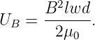 | (17.27) |
The volume between the inductor plates is just dlw, so again we can write an energy density, this time for the magnetic field:
 | (17.28) |
Though we only proved this equation for the magnetic field inside a parallel plate inductor, it turns out to be true for any magnetic field.
The total energy density is just the sum of the electric and magnetic energy densities:
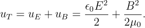 | (17.29) |
In the above discussion of energy we made two assumptions about electric circuits, which consist of electronic components connected by wires:
These are called Kirchhoff’s laws. They are used extensively in electronic circuit design. Figure 17.8 illustrates a typical circuit with a voltage source VS, which may be a battery or generator, and three circuit components. The voltage source provides a potential difference equal to V a - V g, which is equal simply to V a, since we are assuming that V g = 0. (Since the scalar potential is insensitive to an arbitrary additive constant, we can always set the potential at one point in the circuit to zero to simplify our calculations.) The voltage drop across component 1 is V a - V b and the voltage drop across both components 2 and 3 is V b - V g. If the components are resistors, then Ohm’s law can be used to relate the voltage drops across the components to the currents through them. If they are capacitors or inductors, the voltage drop is related respectively to the charge on the capacitor or the time rate of change of current through the inductor. The time rate of change of the charge on the capacitor can be related to the current through the capacitor. The final point in figure 17.8 is that current is conserved at junctions, i. e., i1 = i2 + i3. The methods of algebra (for just resistors) or calculus (if there are capacitors or inductors) can then be used to calculate all currents and voltages.
It is important to realize that Kirchhoff’s laws are only approximations that hold when the currents and potentials in a circuit change slowly with time. For steady currents and constant potentials they are precisely true, since imbalances in charge entering and leaving a junction between devices would result in the indefinite buildup of charge in the junction with time and therefore an increasing electrostatic potential, which would violate the steady state assumption. Furthermore, a non-zero EMF around a closed loop would result in net acceleration of charge around the loop and a constantly increasing current.
If currents and potentials are changing with time, Kirchhoff’s laws are approximately valid only if the capacitance, inductance, and resistance of the wires connecting circuit elements are much smaller than the capacitance, inductance, and resistance of the circuit elements themselves. For very high frequency operation, the effects of these “parasitic” properties are not small and must be included in the design of the circuit.
as shown in figure 17.10. Hint: In the first case the voltage drop across the resistors is the same, in the second, the current through the resistors is the same. Recall that Ohm’s law relates the current through a device to the voltage drop across it. (If you already know the answers, derive them; don’t just write them down.)
The battery produces a voltage difference V , but also may be thought of as having a small internal resistance R.
You may ignore the effect of the current in creating an additional magnetic field.
To begin our study of matter we discuss experiments in the late 19th and early 20th centuries that led to proof of the existence of atoms and their constituents. We then introduce a fundamental idea about the scattering of waves using the diffraction of light by small particles as a prototype. The famous Geiger-Marsden experiment that led to the idea of the atomic nucleus is discussed. Finally, we examine some of the crucial experiments done with modern particle accelerators and the physical principles behind them.1
From the time of the ancient Greeks there have been debates about the ultimate nature of matter. One of these debates is whether matter is infinitely divisible or whether it consists of fundamental building blocks that are themselves indivisible. However, it wasn’t until the late 19th century that real progress began to be made on this question.
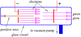
____________________________
Advancements in our understanding of matter have largely been coupled to the development of machines to accelerate atomic and sub-atomic particles. The original accelerator was developed in the 19th century and is called the Crookes tube.
J. J. Thomson measured the charge to mass ratio for both electrons and positive ions in the Crookes tube in the following way: If a potential difference Δϕ is applied between the electrodes, then by energy conservation a particle of charge q starting from rest will acquire a kinetic energy moving from electrode to electrode of K = mv2∕2 = qΔϕ. Solving for v, we find v = (2qΔϕ∕m)1∕2. If a magnetic field B is then imposed normal to the electron beam after it has passed the positive electrode, the beam bends with a radius of curvature of R = mv∕(qB). Since R and B are known, the charge to mass ratio can be computed by eliminating v and solving for q∕m: q∕m = 2Δϕ∕(BR)2. Thomson found that positive ions typically had charge to mass ratios several thousand times smaller than the electrons. Furthermore, the ions were positively charged, while the electrons were negatively charged. If the ions and the electrons have electrical charges equal in magnitude (plausible, since the ions are neutral atoms with at least one electron removed), the ions have to be much more massive than the electrons.
Robert Millikan made the first direct measurement of electric charge. He did this by suspending electrically charged oil drops in a known electric field against gravity. The size of an oil drop is directly measured using a microscope, leading to a calculation of its mass, and hence the gravitational force, mg. This is then balanced against the electric force, qE, leading to q = mg∕E. Occasionally an oil drop loses an electron due to photoelectric emission caused by photons from an ultraviolet lamp. This disrupts the force balance, and causes the oil drop to move up or down. If the electric field is quickly adjusted, this motion can be arrested. The change in the charge can be related to the change in the electric field: Δq = mgΔ(1∕E). If only a single electron is emitted, then Δq is equal to the electronic charge.
Between the work of Thomson and Millikan, the masses and the charges of sub-atomic particles were accurately measured for the first time. Ironically, this work also showed that the “atom”, which means “indivisible” in Greek, in fact isn’t. Atoms consist of positive charges with large mass, or protons, in conjunction with low mass electrons of negative charge. Electrons and protons have opposite charges, so they attract each other to form atoms in this picture.
Geiger and Marsden did an experiment that strongly suggested that atoms consist of very small, positively charged atomic nuclei, surrounded by a cloud of circling, negatively charged electrons. This is called the Rutherford model of the atom after Ernest Rutherford.
Chadwick completed our picture of the atom with the discovery of a neutral particle of mass comparable to the proton, called the neutron. The neutron is a constituent of the atomic nucleus along with the proton. The number of protons in a nucleus is denoted Z while the number of neutrons is N. We define A = Z + N to be the total number of nucleons (protons plus neutrons). The parameter Z is often called the atomic number while A is called the atomic mass number.
Marie and Pierre Curie and Henri Becquerel were the first to discover a more fundamental divisibility of atoms in the form of the radioactive decay, though the implications of their results did not become clear until much later. Radioactive decay of atomic nuclei comes in three common forms: alpha, beta, and gamma decay. Alpha decay is the spontaneous emission of a helium-4 nucleus, called an alpha particle by a heavy nucleus such as uranium or radium. The alpha particle consists of two protons and two neutrons, so the emission decreases both Z and N by 2. Beta decay is the emission of an electron or its antiparticle, the positron, by a nucleus, with an accompanying change in the electric charge of the nucleus. For electron emission Z increases by 1 while N decreases by 1. The opposite occurs for positron emission. Gamma decay is the emission of a high energy photon by a nucleus. The values of Z and N remain unchanged. The energy released by these decays is typically of order a few million electron volts.
Of the three forms of decay, beta decay is the most interesting, since it involves the transformation of one sub-atomic particle into another. In the case of neutron decay, a neutron is converted into a proton, an electron, and an antineutrino. For proton decay, a proton becomes a neutron, a positron, and a neutrino. (Only the neutron form occurs for an isolated particle. However, the energetics inside atomic nuclei can result in either form, depending on the nucleus in question.) The neutrino is one of the great theoretical predictions of modern physics. Careful studies of beta decay, which at the time was thought to result only in the emission of a proton and an electron for the neutron form of the reaction, showed apparent non-conservation of energy and angular momentum. Rather than accept this rather unpalatable conclusion, Wolfgang Pauli proposed that a third particle named a neutrino, or little neutral particle, is emitted in the decay, thus accounting for the missing energy and angular momentum. The presumed electrical neutrality of the particle explained the difficulty of detecting it. Over 25 years passed before Frederick Reines and Clyde Cowan from Los Alamos observed this elusive particle.
The three forms of radioactive decay are associated with three of the four known fundamental forces of nature. Gamma decay is electromagnetic in nature, while alpha decay involves the breaking of bonds produced by the nuclear or strong force. Beta decay is a manifestation of the so-called weak force. (The fourth force is gravity, which plays a negligible role on the sub-atomic scale, as far as we know.)
Beta decay gives us a strong hint that even particles such as protons and neutrons, which make up atomic nuclei, are not “atomic” in the sense of the original Greek, since neutrons can change into protons in beta decay and vice versa. We now have excellent evidence that protons, neutrons, and many other sub-nuclear particles are made up of particles called quarks. Quarks and electrons are currently thought to be fundamental in that they are supposedly indivisible, and are hence the true “atoms” of the universe. However, who knows, perhaps someday we will discover that they too are composed of even more fundamental constituents!
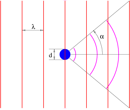
____________________________
Sometimes at night one sees a diffuse disk of light around the moon if it happens to be shining through a thin layer of cloud. This disk consists of light diffracted by the water or ice particles in the cloud. The diameter of the disk contains information about the size of the cloud particles doing the diffraction. In particular, if the particles have diameter d and the light has wavelength λ, then the diffraction half-angle shown in figure 18.2 is approximately
 | (18.1) |
This equation comes from the problem of passage of light through a hole or slit of diameter or width d. This problem was treated in the chapter on waves, and the above formula was concluded to hold in that case. One can think of the diffraction of light by a particle to be the linear superposition of a plane wave minus the diffraction of light by a hole in a mask, as illustrated in figure 18.2. The angular spread of the diffracted light is the same in both cases.
The interesting point about equation (18.1) is that the opening angle of the diffraction cone is inversely proportional to the diameter of the diffracting particles. Thus, for a given wavelength, smaller particles cause diffraction through a wider angle.
Note that when the wavelength exceeds the diameter of the particle by a significant amount, equation (18.1) fails, since scattering through an angle greater than π doesn’t make physical sense. In this case the diffracted photons tend to be isotropic, i. e., they are scattered with equal probability into any direction.
If one wishes to measure the size of an object by observing the diffraction of a wave around the object, the lesson is clear; the wavelength of the wave must be less than or equal to the dimensions of the object — otherwise the scattering of the wave by the object is largely isotropic and equation (18.1) yields no information. Since wavelength is inversely related to momentum by the de Broglie relationship, this condition implies that the momentum must satisfy
 | (18.2) |
in order that the size of an object of diameter d be resolved.
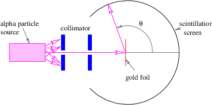
____________________________
In 1908 Hans Geiger and Ernest Marsden, working with Ernest Rutherford of the Physical Laboratories at the University of Manchester, measured the angular distribution of alpha particles scattered from a thin gold foil in an experiment illustrated in figure 18.3. In order to understand this experiment, we need to compute the de Broglie wavelength of alpha particles resulting from radioactive decay. Typical alpha particle kinetic energies are of order 5 MeV = 8 × 10-13 J. Since the alpha particle consists of two protons and two neutrons, its mass is about Mα = 6.7 × 10⁻²⁷ kg. This implies a velocity of about v = 1.1 × 10⁷ m s-1, a momentum of about p = mv = 7.4 × 10⁻²⁰ N s, and a de Broglie wavelength of about λ = h∕p = 9.0 × 10⁻¹⁵ m.
Other evidence indicates that atoms have dimensions of order 10-10 m, so the de Broglie wavelength of an alpha particle is about a factor of 104 smaller than a typical atomic dimension. Thus, the typical diffraction scattering angle of alpha particles off of atoms ought to be very small, of order α = λ∕(2d) ≈ 10-4 radian ≈ 0.01∘.
Imagine the surprise of Geiger and Marsden when they found that while most alpha particles suffered only small deflections when passing through the gold foil, a small fraction of the incident particles scattered through large angles, some in excess of 90∘!
![]()
____________________________
Ernest Rutherford calculated the probability for an alpha particle, considered to be a positive point charge, to be scattered through various angles by a stationary atomic nucleus, assumed also to be a positive point charge. The calculation was done classically, though interestingly enough a quantum mechanical calculation gives the same answer. The relative probability for scattering with a momentum transfer to the alpha particle of q is proportional to |q|-4 ≡ q-4 according to Rutherford’s calculation. (Do not confuse this q with charge!) As figure 18.4 indicates, a larger momentum transfer corresponds to a larger scattering angle. The maximum momentum transfer for an incident alpha particle with momentum p is 2|p|, or just twice the initial momentum. This corresponds to a head-on collision between the alpha particle and the nucleus followed by a recoil of the alpha particle directly backwards. Since this collision is elastic, the kinetic energy of the alpha particle after the collision is approximately the same as before, as long as the nucleus is much more massive than the alpha particle.
Rutherford’s calculation agreed quite closely with the experimental results of Geiger and Marsden. Though the probability for scattering through a large angle is small even in the Rutherford theory, it is still much larger than would be expected if there were no small scale atomic nucleus.
Earlier we indicated that particles interacted with each other via the exchange of a virtual intermediary particle that interchanges energy, momentum, and other physical properties between the interacting particles. This idea originated with the Japanese physicist Hideki Yukawa in 1935 in an effort to understand the forces between nucleons. Yukawa hypothesized that the force that holds nucleons together is associated with the exchange of a boson, i. e., a particle with integer spin, with rest energy mc2 ≈ 100 MeV. The range of this force at low momentum transfers is I ≈ℏ∕(mc) ≈ 2 × 10-15 m, or comparable to the observed size of an atomic nucleus.
In 1947 two new particles were discovered in cosmic rays, the negatively charged muon with a rest energy of 106 MeV, and the pion, which comes in three varieties, the π+, the π-, and the π0, which respectively have positive, negative, and zero charge. The rest energies of the π+ and π- are 140 MeV while that of the π0 is 135 MeV. All of these particles are unstable in that they decay into other, more stable particles in a tiny fraction of a second. In particular, the negative pion decays into a muon and an antineutrino, while the neutral pion decays into two gamma rays, or high energy photons. The antineutrino that results from pion decay is actually distinct from the antineutrino emitted in nuclear beta decay; it is called the mu antineutrino since it is associated with the muon in the same way that the antineutrino in beta decay is associated with the electron. To further distinguish between the two, the latter is called the electron antineutrino. The muon itself decays into an electron, a mu neutrino, and an electron antineutrino.
The muon and its associated neutrino are rather peculiar. In all respects except mass, the muon appears to be identical to the electron. The physicist I. I. Rabi is reputed to have responded “Who ordered that?” upon learning of the properties of the muon. Furthermore, the electron neutrino only interacts with the electron and the muon neutrino only interacts with the muon. This is the first hint that elementary particles occur in families that appear to be replicated at higher energies.
Since the muon is a fermion with spin 1∕2, it can’t be Yukawa’s intermediary particle since all intermediary particles are bosons with integral spin. Furthermore, as with the electron, it is not subject to the nuclear force. The pions are more promising candidates for being intermediary particles of the nuclear force, since they are bosons with spin 0. However, as we shall see, the situation is more complex than Yukawa imagined, and the force between nucleons cannot be so simply treated. However, Yukawa’s idea of intermediary particle exchange lives on in today’s theories of sub-nuclear particles.
Soon after the discovery of muons and pions in cosmic rays, a whole plethora of unstable particles was uncovered. Central to these discoveries was the particle accelerator. In these devices, charged particles, typically electrons or protons, are accelerated to high energy and then smashed into a target. Detectors of various sorts are used to examine the particles created by the collisions of the accelerated particles and the atomic nuclei with which they collide. Sometimes an elastic collision occurs, in which the accelerated particle simply “bounces off” of the target particle, transferring a good bit of its momentum to this sparticle. However, under many circumstances the collision results in the production of new particles that didn’t exist before the collision. This is referred to as an inelastic collision.
The simplest type of target is liquid hydrogen since the nucleus consists of a single proton. The orbital electrons of the target atoms are so light that they are generally just “brushed aside” without greatly affecting the trajectories of the accelerated particles. However, a variety of targets are used under different circumstances.
In the late 1950s and early 1960s Robert Hofstadter of Stanford University extended the Geiger-Marsden experiment to much shorter de Broglie wavelengths using high energy electrons from an accelerator, rather than alpha particles, as the probe. The type of results obtained by Hofstadter are shown in figure 18.5. After accounting for some effects having to do with the electron spin, these experiments should agree with the Rutherford formula if the nucleus is truly a point particle. This is shown by the solid line in figure 18.5. However, the actual results (dashed line) show probabilities that drop off more rapidly with increasing momentum transfer q than is predicted by the Rutherford model.
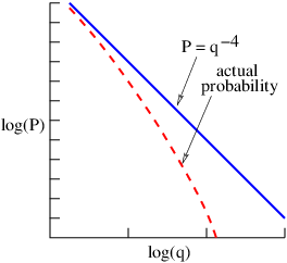
____________________________
These results are related to the fact that the nucleus is actually of finite size. The diffraction effects discussed in the section on the scattering of moonlight come into play here, in that little scattering takes place for scattering angles larger than roughly λ∕(2d), where λ is the de Broglie wavelength of the probing particle and d is the diameter of the target. For a small scattering angle (which we now call θ), it is clear from figure 18.4 that
 | (18.3) |
where p is the momentum of the incident electron and q is the momentum transfer. If qmax is the maximum momentum transfer for which there is significant scattering, then we can write
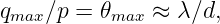 | (18.4) |
where the factor of 2 in the denominator on the right side has been dropped since this is an approximate analysis. However, since λ = h∕p, we find that
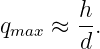 | (18.5) |
Thus, the momentum transfer for which the dashed line in figure 18.5 becomes small compared to the solid line gives us an immediate estimate of the diameter of an atomic nucleus: d ≈ h∕qmax. The results obtained by Hofstadter show that nuclear diameters are typically a few times 10-15 m.
More than just size information can be extracted from this analysis. Hofstadter’s experiments also led to a great deal of information about the internal structure of atomic nuclei.
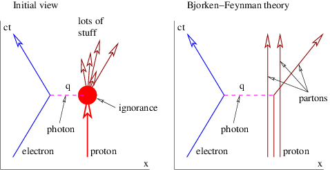
____________________________
The construction of the Stanford Linear Accelerator Center (SLAC), which accelerates electrons up to 40 GeV, allowed experiments like Hofstadter’s to be carried out at much higher energies. At these energies, many of the collisions between electrons and protons and neutrons are inelastic — generally a great mess of short-lived particles is spewed out, and are very difficult to interpret. However, the so-called deep inelastic collisions, where the electron scatters through a large angle and therefore transfers a large momentum, q, to the proton, yield very interesting results. In particular, these collisions occur essentially with a probability proportional to q-4 — just as in the Geiger-Marsden experiment!
The electron is a point particle as far as we know. However, previous experiments showed the proton to have a finite size, of order 10-15 m. Therefore, the scattering probability should drop off more rapidly with increasing momentum transfer q than with q-4, as in the earlier Hofstadter experiments.
James Bjorken and Richard Feynman showed a way out of this dilemma. They proposed that the proton actually consists of a small number of point particles bound together by weakly attractive forces. A sufficiently energetic photon is able to knock a single one of these particles out of the proton, as illustrated in the right panel of figure 18.6. This leads to a subsequent set of reactions that produce the profusion of particles seen in the left panel of this figure. Feynman called the particles that make up the proton partons. However, we now know that they are actually quarks, spin 1/2 particles with fractional electronic charge that are thought to be the fundamental building blocks of matter, and gluons, the massless spin 1 intermediary particles that carry the strong force.
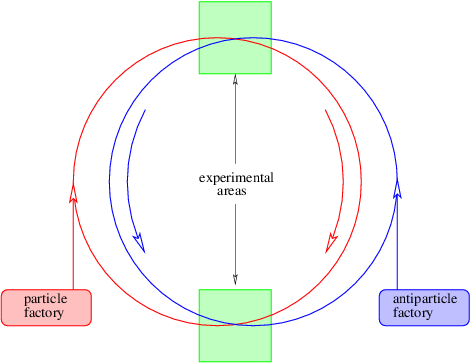
____________________________
An alternate way to create interesting collisions is to crash particles and antiparticles of the same energy into each other. This is done via a storage ring, as shown in figure 18.7. A set of magnets forces particles and antiparticles (which have opposite charges) to move in opposing circles within a high vacuum. The circles are slightly offset so that the beams cross at only two points. Collisions occur at these points and are observed by various types of experimental equipment.
An alternate type of collider has two storage rings that intersect at only one point. This type of system can be used to collide particles of the same type together, e. g., protons colliding with protons.
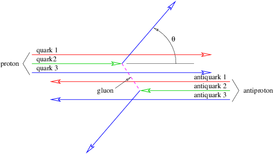
____________________________
If collisions occur by the exchange of a single intermediary particle of zero mass between point particles, the q-4 dependence of the collision probability on momentum transfer will occur in proton-antiproton collisions as in the Geiger-Marsden experiment. However, if the colliding particles are not point particles, a form factor that decreases for increasing momentum transfer will occur as with the Hofstadter experiments.
When collisions between protons and antiprotons of a few hundred GeV are arranged, certain types of events called two-jet events are recorded. In these events, two jets, each containing many particles, are emitted in opposite directions at wide angles (i. e., with large momentum transfer) from the colliding beams. Furthermore, these jets show a probability distribution as a function of momentum transfer very close to q-4. This indicates that the colliding particles are point-like, at least down to the minimum spatial resolutions available to today’s accelerators.
According to the Bjorken-Feynman parton model of the proton, the collision between highly energetic protons and antiprotons should operate as shown in figure 18.8. The actual collision is between individual partons. Figure 18.8 illustrates the collision between a quark in the proton and an antiquark in the antiproton. The result of this interaction is the scattering of these particles out of the incident particles, resulting ultimately in a two jet event as described above.
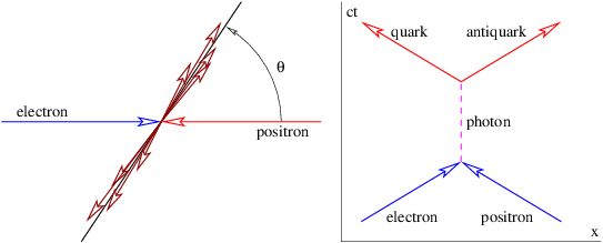
____________________________
Two-jet events can also be created by the collision of high energy electrons and positrons. Figure 18.9 shows how this process is thought to work. The annihilation of the electron and positron results in a virtual photon, which in turn decays into a quark-antiquark pair. The quarks then produce the jets. These results suggest that quarks can indeed occur outside of protons, at least if they occur in quark-antiquark pairs.
We have examined a selected set of experiments performed over the last 100 years. Though complicated in detail, we have seen that they can be understood in their essence using one idea, namely the uncertainty principle. This principle underlies the diffraction angle formula and also turns out (in an argument that we have not made) to be central to the q-4 dependence of scattering probability for point particles. For momentum transfers of order 1000 GeV/c, we are able to probe spatial scales of order 10-17 m, or a factor of 100-500 less than the scale of the atomic nucleus. Even on this scale it appears that both the electron and the quark act like point particles. They thus appear to be the ultimate “atoms” of matter in the original sense of the word. However, it is possible that experiments at even higher momentum transfers would show the electron or the quark to have some kind of internal structure. Perhaps this heirarchy of structure, of which we have noted the atom, the atomic nucleus, nucleons, and quarks, goes on forever.
Hint: Use the non-relativistic kinetic energy and check whether this assumption is valid in retrospect.
Hint: Recall that the smallest feature resolvable by a wave is approximately the wavelength of that wave.
Hint: These calculations are relativistic, since the rest energy of the proton is about 0.9 GeV.
In this chapter we investigate the structure of atoms. However, before we can understand these, we first need to review some facts about angular momentum in quantum mechanics.
As we learned earlier, angular momentum is quantized in quantum mechanics. We can simultaneously measure only the magnitude of the angular momentum vector and one component, usually taken to be the z component. Measurement of the other two components simultaneously with the z component is forbidden by the uncertainty principle.
The magnitude of the orbital angular momentum of an object can take on the values |L| = [l(l + 1)]1∕2ℏ where l = 0, 1, 2,…. The z component can likewise equal Lz = mℏ where m = -l,-l + 1,…,l.
Particles can have an intrinsic spin angular momentum as well as an orbital angular momentum. The possible values for the magnitude of the spin angular momentum are |S| = [s(s + 1)]1∕2ℏ and the z component of the spin angular momentum Sz = msℏ where ms = -s,-s + 1,…,s. Spin differs from orbital angular momentum in that the spin can take on half-integer as well as integer values: s = 0, 1∕2, 1, 3∕2,… are possible spin quantum numbers.
Spin is an intrinsic, unchangeable quantity for an elementary particle. Particles with half-integer spins, s = 1∕2, 3∕2, 5∕2,…, are called fermions, while particles with integer spins, s = 0, 1, 2,… are called bosons. Fermions can only be created or destroyed in particle-antiparticle pairs, whereas bosons can be created or destroyed singly.
We learned in quantum mechanics that a particle is represented by a wave, ψ(x,y,z,t), the absolute square of which gives the relative probability of finding the particle at some point in spacetime. If we have two particles, then we must ask a more complicated question: What is the relative probability of finding particle 1 at point x1 and particle 2 at point x2? This probability can be represented as the absolute square of a joint wave function ψ(x1,x2), i. e., a single wave function that represents both particles. If the particles are not identical (say, one is a proton and the other is a neutron) and if they are not interacting with each other via some force, then the above wave function can be broken into the product of the wave functions for the individual particles:
 | (19.1) |
In this case the probability of finding particle 1 at x1 and particle 2 at x2 is just the absolute square of the joint wave amplitude: P(x1,x2) = P1(x1)P2(x2). This is consistent with classical probability theory.
The situation in quantum mechanics when the two particles are identical is quite different. If P(x1,x2) is, say, the probability of finding one electron at x1 and another electron at x2, then since we can’t tell the difference between one electron and another, the probability distribution cannot change if we switch the electrons. In other words, we must have P(x1,x2) = P(x2,x1). There are two obvious ways to make this happen: Either ψ(x1,x2) = ψ(x2,x1) or ψ(x1,x2) = -ψ(x2,x1).
It turns out that the wave function for two identical fermions is antisymmetric to the exchange of particles whereas for two identical bosons it is symmetric. In the special case of two non-interacting particles, we can construct the joint wave function with the correct symmetry from the wave functions for the individual particles as follows:
 | (19.2) |
for fermions and
 | (19.3) |
for bosons.
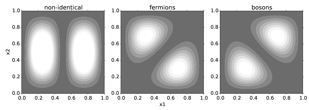
____________________________
Figure 19.1 shows the joint probability distribution for two particles in different energy states in an infinite square well: P(x1,x2) = |ψ(x1,x2)|2. Three different cases are shown: non-identical particles, identical fermions, and identical bosons. Notice that the probability of finding two fermions at the same point in space, i. e., along the diagonal dotted line in the center panel of figure 19.1, is zero. This follows immediately from equation (19.2), which shows that ψ(x1,x2) = 0 for fermions if x1 = x2. Notice also that if two fermions are in the same energy level (say, the ground state of the one-dimensional box) so that ψ1(x) = ψ2(x), then ψ(x1,x2) = 0 everywhere. This demonstrates that the two fermions cannot occupy the same state. This result is called the Pauli exclusion principle.
On the other hand, bosons tend to cluster together. Figure 19.1 shows that the highest probability in the joint distribution occurs along the line x1 = x2, i. e., when the particles are colocated. This tendency is accentuated when more particles are added to the system. When there are a large number of bosons, this tendency creates what is called a Bose-Einstein condensate in which most or all of the particles are in the ground state. Bose-Einstein condensation is responsible for such phenomena as superconductivity in metals and superfluidity in liquid helium at low temperatures.
The Rutherford model of the atom has electrons moving in orbit around a small, positively charged nucleus. Thus, in general electrons have both angular momentum and magnetic dipole moments. These magnetic moments are important for understanding the magnetic properties of matter. Even though the Rutherford model has been superseded by quantum mechanics, the classically derived relationship between angular momentum and magnetic moment remains useful.
Imagine a particle with mass M and charge q moving in a circle of radius R with speed v. Treating the motion of this particle classically, with speed much less than the speed of light, the orbital angular momentum of the particle is L = MvR. The time for the particle to make one revolution is T = 2πR∕v, so the circular current represented by this moving charge is i = q∕T = qv∕(2πR). The magnetic moment generated by this circular current is the current times the area of the circle, or m = iA = iπR2. The ratio of the magnetic moment to the angular momentum of the particle
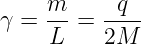 | (19.4) |
is called the gyromagnetic ratio.
This equation turns out to be generally true, even if particles are not moving in circular orbits. However, elementary particles have an intrinsic angular momentum that has nothing to do with orbital motion. For the electron in particular, the gyromagnetic ratio is (to within a tenth of a percent)
 | (19.5) |
where e is the charge on the electron and Me is its mass, or twice the gyromagnetic ratio of the electron in orbital motion. (Technically, the gyromagnetic ratio of particles with negative charge is negative, though this sign is often ignored.) Since the spin angular momentum of the electron is ℏ∕2, the intrinsic magnetic moment associated with the electron spin is
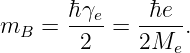 | (19.6) |
This is sometimes called the Bohr magneton, hence the subscripted B. The factor of 2 missing from equation (19.5) in comparison to equation (19.4) results from relativistic factors, but the derivation is rather complex, so we will not present it here.
Magnetic dipoles from orbital and spin angular momenta have important practical consequences; they are central to the phenomena of paramagnetism and ferromagnetism. Paramagnetism occurs when atoms have an odd number of electrons, which means that the angular momentum of these electrons does not add up to zero (see next chapter). In this case, there is a net magnetic dipole moment for each atom. If a magnetic field is imposed, this dipole tends to align with the magnetic field, which in turn reinforces the imposed field, resulting in a stronger total field. If the imposed magnetic field is taken away, the atoms reorient themselves randomly, resulting in zero field.
A few materials, such as iron, exhibit a more complex phenomenon called ferromagnetism. In this case the imposition of an external magnetic field causes very strong dipole alignment effects to the point where interactions between the newly aligned dipoles prevent the reversion to random orientation when the imposed field is removed. “Permanent” magnets may be created this way. As the temperature increases, the thermal jiggling of atoms increases in proportion. If this jiggling becomes strong enough, the tendency of neighboring dipoles to maintain a common orientation is overcome and the material becomes paramagnetic. The temperature at which this occurs for a particular material is called the Curie temperature.
If there are no unpaired electrons in a material, then there are no pre-existing dipoles to align. However, the magnetic field still distorts the motions of electrons via the Lorentz force. The result is the production of induced magnetic dipoles that anti-align with the field, as happens with the electrons in a plasma. The resulting induced magnetic field opposes the original field, resulting in a total field that is less than originally imposed. Such a material is called diamagnetic.
The hydrogen atom consists of an electron and a proton bound together by the attractive electrostatic force between the negative and positive charges of these particles. Our experience with the one-dimensional particle in a box shows that a spatially restricted particle takes on only discrete values of the total energy. This conclusion carries over to arbitrary attractive potentials and three dimensions.
The energy of the ground state can be qualitatively understood in terms of the uncertainty principle. A particle restricted to a region of size a by an attractive force will have a momentum equal at least to the uncertainty in the momentum predicted by the uncertainty principle: p ≈ℏ∕a. This corresponds to a kinetic energy K = mv2∕2 = p2∕(2m) ≈ℏ2∕(2ma2). For the particle in a box there is no potential energy, so the kinetic energy equals the total energy. Comparison of this estimate with the computed ground state energy of a particle in a box of length a, E1 = ℏ2π2∕(2ma2), shows that the estimate differs from the exact value by only a numerical factor π2.
We can make an estimate of the ground state energy of the hydrogen atom using the same technique if we can somehow take into account the potential energy of this atom. Classically, an electron with charge -e moving in a circular orbit of radius a around a proton with charge e at speed v must have the centripetal acceleration multiplied by the mass equal to the attractive electrostatic force, mv2∕a = e2∕(4πϵ 0a2), where m is the electron mass. (The proton is so much more massive than the electron that we can assume it to be stationary.) Multiplication of this equation by a∕2 results in
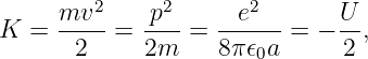 | (19.7) |
where U is the (negative) potential energy of the electron and K is its kinetic energy. Solving for U, we find that U = -2K. The total energy E is therefore related to the kinetic energy by
 | (19.8) |
Since the total energy is negative in this case, and since U = 0 when the electron is infinitely far from the proton, we can define a binding energy that is equal to minus the total energy:
 | (19.9) |
The binding energy is the minimum additional energy that needs to be added to the electron to make the total energy zero, and thus to remove it to infinity. Equation (19.9) is called the virial theorem, and it is even true for non-circular orbits if the energies are properly averaged over the entire trajectory.
Proceeding as before, we assume that the momentum of the electron is p ≈ℏ∕a and substitute this into equation (19.7). Solving this for a ≡ a0 yields an estimate of the radius of the hydrogen atom:
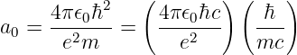 | (19.10) |
This result was first obtained by the Danish physicist Niels Bohr, using another method, in an early attempt to understand the quantum nature of matter.
The grouping of terms by the large parentheses in equation (19.10) is significant. The dimensionless quantity
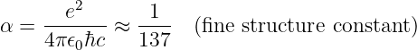 | (19.11) |
is called the fine structure constant for historical reasons. However, it is actually a fundamental measure of the strength of the electromagnetic interaction. The Bohr radius can be written in terms of the fine structure constant as
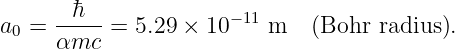 | (19.12) |
The binding energy predicted by equations (19.7) and (19.9) is
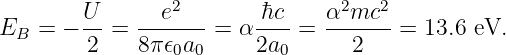 | (19.13) |
The binding energy between the electron and the proton is thus proportional to the electron rest energy multiplied by the square of the fine structure constant.
The above estimated binding energy turns out to be precisely the ground state binding energy of the hydrogen atom. The energy levels of the hydrogen atom turn out to be
 | (19.14) |
where n is called the principal quantum number of the hydrogen atom.
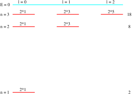
____________________________
The energy levels of the hydrogen atom whose energies are given by equation (19.14) are actually degenerate, in that each energy has more than one state associated with it. Three extra degrees of freedom are associated with angular momentum, expressed by the quantum numbers l, m, and ms. For energy level n, the orbital angular momentum quantum number can take on the values l = 0, 1, 2,…,n - 1. Thus, for the ground state, n = 1, the only possible value of l is zero. For a given value of l, there are 2l + 1 possible values of the orbital z component quantum number, m = -l,-l + 1,…,l. Finally, there are two possible values of the spin orientation quantum number, ms. Thus, for the nth energy level there are
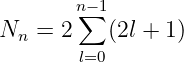 | (19.15) |
states. In particular, for n = 1, 2, 3,…, we have Nn = 2, 8, 18,…. This is summarized in figure 19.2.
These results have implications for the character of atoms with more than one proton in the nucleus. Let us imagine how such atoms might be built. The binding energy of a single electron in the ground state of a nucleus with Z protons is Z2 multiplied by the binding energy of the electron in the ground state of a hydrogen atom. If the force between electrons can be ignored compared to the force between an electron and the nucleus (a very poor but initially useful assumption that we will discuss below), then we could construct an atom by dropping Z electrons one by one into the potential well of the nucleus. The Pauli exclusion principle prevents all of these electrons from falling into the ground state. Instead, the available states will fill in order of lowest energy first until all Z electrons are added and the atom becomes electrically neutral. From figure 19.2 we see that Z = 2 fills the n = 1 levels with two electrons, one spin up and one spin down, both with zero orbital angular momentum. For Z = 10 the n = 2 levels fill such that two electrons have l = 0 and six have l = 1.
As electrons are added to an atom, previous electrons tend to shield subsequent electrons from the nucleus, since their negative charge partially compensates for the nuclear positive charge. Thus, binding energies are considerably less than would be expected on the basis of the non-interacting electron model. Furthermore, the binding energies for states with higher orbital angular momentum are smaller than those with lower values, since electrons in these states tend to be more effectively shielded from the nucleus by other electrons. This effect becomes sufficiently important at higher Z to disrupt the sequence in which states are filled by electrons — sometimes level n + 1 states with low l start to fill before all the level n states with large l are full. Accurate calculations of atomic properties in which electron-electron interactions are taken into account are possible, but are computationally expensive.
The best evidence for atomic energy levels comes from the emission of light by atoms in a gas at low pressure. If the atoms are put in an excited state by some mechanism, say, collisions with energetic electrons accelerated by a potential difference between electrodes, then light is emitted at particular frequencies called spectral lines. These frequencies can be separated by a device called a spectroscope. Spectroscopes use either a prism or a diffraction grating and ancillary optics to make the separation visible to the eye.
The frequency of a spectral line is equal to the energy difference between two states divided by Planck’s constant. This is a consequence of the conservation of energy — the energy released when an atom undergoes a transition from a state with energy E2 to a state with energy E1 is just the difference between these energies. The frequency of the emitted photon is then derived from the Planck formula. In terms of the angular frequency,
 | (19.16) |
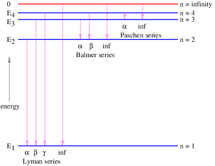
____________________________
Figure 19.3 shows the possible transitions between the lowest four energy levels of hydrogen plus the ionized state in which the electron is initially a large distance from the hydrogen nucleus. Transitions from any state to the ground state form a series called the Lyman series, while transitions to the first excited state are called the Balmer series, transitions to the second excited state are called the Paschen series, and so on. Within each series, increasing frequencies are labeled using the Greek alphabet, so the transition from n = 2 to n = 1 is called the Lyman-α spectral line, etc.
Atoms can absorb as well as emit radiation. For instance, if hydrogen atoms in the ground state are bombarded with photons of energy equal to the energy difference between the ground state and some excited state, some of the atoms will absorb these photons and undergo transitions to the excited state. If white light (i. e., many photons with a continuous distribution of frequencies) irradiates such atoms, just those photons with the right energies will be absorbed. Examination of the light with a spectroscope after it passes through a gas of atoms will show absorption lines where the photons with the critical energies have been removed. This is one of the main ways in which astrophysicists learn about the elemental constitution of stars and interstellar gases.
Atoms in excited states emit photons spontaneously. However, a process called stimulated emission is also possible. This occurs when a photon with energy equal to the difference between two atomic energy levels interacts with an atom in the higher energy state. The amplitude for this process is equal to the spontaneous emission amplitude times n + 1, where n is the number of incident photons with energy equal to the energy of the photon which would be spontaneously emitted. If a beam of photons with the right energy shines on atoms in an excited state, the beam will gain energy at a rate that is proportional to the initial intensity of the beam. For intense beams, this stimulated emission process overwhelms spontaneous emission and a large amount of energy can be rapidly extracted from the excited atoms. This is how a laser works.

Hint: In each case there are six terms corresponding to the six permutations of x1, x2, and x3. Exchanging any two particles leaves ψ unchanged for bosons but changes the sign for fermions.
Hint: If the outgoing particles (but not the incoming particles) are interchanged, how does the apparent deflection angle change?
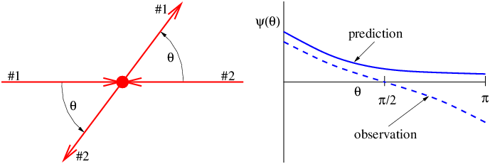
_____________________________________
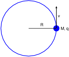
_____________________________________
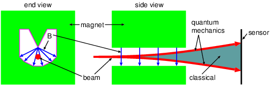
_____________________________________
In this chapter we learn about the most fundamental known particles of the universe, and how they act as building blocks for everything that we know. The theory describing this scheme is called the standard model. Speculations exist about possible, more fundamental structures in the universe, such as the constructs of string theory. However, with the standard model we have reached the frontier of what is known with any degree of certainty.
The standard model of hadrons and leptons is a united set of quantum mechanical theories encompassing electromagnetism; the weak force, which is responsible for beta decay; and the strong force, which holds atomic nuclei together. Before investigating the standard model, we need to describe the state of affairs previous to its development. The creation of high energy particle accelerators led to the discovery of a plethora of particles in addition to those already known. These particles fall into the following categories:
We will discover additional intermediary particles in our discussion of the standard model.
The standard model postulates that all known particles are either fundamental point particles or are composed of fundamental point particles according to a remarkably small set of rules. Just as atoms are bound states of atomic nuclei and electrons, atomic nuclei are bound states of protons and neutrons. Atomic nuclei are discussed in the next section. In this section we delve one step deeper in the heirarchy of the universe. We now believe that all hadrons are actually bound states of fundamental spin 1/2 particles called quarks. Whereas all other known charged particles have an electric charge equal to an integer multiple of ±e where e is the proton charge, quarks have electric charges equal to either -e∕3 or +2e∕3. Leptons themselves are considered to be fundamental, so the leptons and the quarks form the basic building blocks of all matter in the universe.
Quarks are subject to electromagnetic forces via their charge, but interact most strongly via the so-called strong force. The strong force is carried by massless, uncharged, spin 1 bosons called gluons.
| Type | Charge | Rest energy | s | c | b | t |
| down (d) | -1∕3 | 0.333 | 0 | 0 | 0 | 0 |
| up (u) | +2∕3 | 0.330 | 0 | 0 | 0 | 0 |
| strange (s) | -1∕3 | 0.486 | -1 | 0 | 0 | 0 |
| charm (c) | +2∕3 | 1.65 | 0 | +1 | 0 | 0 |
| bottom (b) | -1∕3 | 4.5 | 0 | 0 | -1 | 0 |
| top (t) | +2∕3 | 176 | 0 | 0 | 0 | +1 |
____________________________
When Murray Gell-Mann and George Zweig first proposed the quark model in 1963, they needed to postulate only three types or flavors of quarks: up, down, and strange. These were sufficient to explain the constitution of all hadrons known at the time. We currently know of six different flavors of quarks. Their properties are listed in table 20.1. The properties charm, topness, and bottomness are analogous to strangeness — these properties are conserved in strong interactions. Weak interactions, discussed in the next section, can turn quarks of one flavor into another flavor. However, the strong and electromagnetic forces cannot do this.
| Type | Charge | Rest energy | Spin | Composition | Mean life |
| proton | +1 | 938.280 | 1/2 | uud | stable |
| neutron | 0 | 939.573 | 1/2 | udd | 898 |
| lambda | 0 | 1116 | 1/2 | uds | 3.8 × 10⁻⁹ |
| delta++ | +2 | 1232 | 3/2 | uuu | 5.6 × 10⁻²⁴ |
| positive pion | +1 | 140 | 0 | ud | 2.6 × 10⁻⁸ |
| negative pion | -1 | 140 | 0 | ud | 2.6 × 10⁻⁸ |
| neutral pion | 0 | 135 | 0 | uu - dd | 8.7 × 10⁻¹⁷ |
| positive rho | +1 | 770 | 1 | ud | 4 × 10-24 |
| positive kaon | +1 | 494 | 0 | us | 1.24 × 10⁻⁸ |
| neutral kaon | 0 | 498 | 0 | ds | 8.6 × 10⁻¹¹ |
| J/psi | 0 | 3097 | 1 | cc | 1.5 × 10⁻²⁰ |
____________________________
Just as the proton and the neutron have antiparticles, so do quarks. Antiquarks of a particular type have strong and electromagnetic charges of the sign opposite to the corresponding quarks. Quarks have baryon number equal to 1∕3, while antiquarks have -1∕3. Thus combining three quarks results in a baryon number equal to 1, while together a quark plus an antiquark have baryon number zero. All baryons are thus combinations of three quarks, while all mesons are combinations of a quark and an antiquark. Table 20.2 lists a sampling of hadrons and some of their properties. Notice that the same combination of quarks can make up more than one particle, e. g., the positive pion and the positive rho. The positive rho may be considered as an excited state of the ud system, while the positive pion is the ground state of this system.
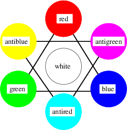
____________________________
Yet to be mentioned is the quantum number color, which has nothing to do with real colors, but has analogous properties. Each flavor of quark can take on three possible color values, conventionally called red, green, and blue. This is illustrated in figure 20.1. Antiquarks can be thought of as having the colors antired, antigreen, and antiblue, also known as cyan, magenta, and yellow. Because of this, the theory of quarks and gluons is called quantum chromodynamics. Counting all color and flavor combinations, there are 6 × 3 = 18 known varieties of quarks.
As in electromagnetism, the strong force has associated with it a “strong charge”, gs. However, this charge is somewhat more complicated than electromagnetic charge in that there are three kinds of strong charge, one for each of the strong force colors. Each color of charge can take on positive and negative values equal to ±gs. As with electromagnetism, positive and negative charges (of the same color) cancel each other. However, in quantum chromodynamics there is an additional way in which charges can cancel. A combination of equal amounts of red, green, and blue charges results in zero net strong charge as well.
The delta++ particle (see table 20.2) is good evidence for the existence of the color quantum number. Since all three u-quarks in the delta++ have spin orientation up, the Pauli exclusion principle would only allow one of these quarks to exist in the ground state if color did not exist, resulting in a much larger mass. As it is, each of the quarks in the delta++ takes on a different value of the color quantum number (red, green, or blue), which means that the Pauli exclusion principle does not prevent them from all from residing in the ground state.
Gluons, the intermediary particles of the strong interaction come in eight different varieties, associated with differing color-anticolor combinations. Since gluons don’t interact via the weak force, there is no flavor quantum number for gluons — quarks of all flavors interact equally with all gluons.
The quark model of matter has led to extensive searches for free quark particles. However, these searches for free quarks have proven unsuccessful. The current interpretation of this result is that quarks cannot exist in a free state, basically because the attractive potential energy between quarks increases linearly with separation. This appears to be related to the fact that gluons, the intermediary particles for the strong force, can interact with each other as well as with quarks. This leads to a series of increasingly complex processes as quarks move farther and farther apart. The result is called quark confinement — apparently, individual quarks can never be observed outside of the confines of the observable particles that contain them.
Confinement works not only on single quarks, but on any “colored” combinations of quarks and gluons, e. g., a red up quark combined with a green down quark. It appears that long range inter-quark forces only vanish for interactions between “white” or “color-neutral” combinations of quarks. This is why only color-neutral combinations of quarks — three quarks of three different colors or a quark-antiquark pair of the same color — are actually seen as observable particles.
The strong equivalent of the fine structure constant is the coupling constant for the strong force:
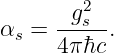 | (20.1) |
Note that αs is dimensionless. The binding energy between quarks is comparable to the rest energies of the quarks themselves. In other words, αs ≈ 1. Furthermore, as we have noted, the potential energy between two quarks appears to increase indefinitely with separation. Though forces exist between color-neutral particles, they are weak and of short range compared to the forces between quarks or colored combinations of quarks. However, they are still relatively strong compared to, say, electromagnetic forces. As we shall see later, these residual strong forces are responsible for nuclear processes.
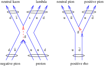
____________________________
Interactions between hadrons can be thought of as resulting from interactions between the individual quarks making up the hadrons. Two sample strong interactions are shown in figure 20.2. Virtual gluons can be emitted and absorbed by quarks much as virtual photons can be emitted and absorbed by electrically charged particles. Particles unstable to strong decay processes (such as the positive rho particle) typically live only about 10-23 s, whereas particles stable to strong decay but unstable to weak decay live of order 10-10 s or longer, depending strongly on how much energy is liberated in the decay. Particles subject to electromagnetic decay processes, such as the neutral pion, take on mean lifetimes intermediate between strong and weak values, typically of order 10-18 s.
| Type | Charge | Rest energy | Mean life |
| electron (e-) | -1 | 0.000511 | stable |
| electron neutrino (νe) | 0 | ≈ 0 | stable |
| muon (μ-) | -1 | 0.106 | 2.2 × 10⁻⁶ |
| mu neutrino (νμ) | 0 | ≈ 0 | stable |
| tau (τ) | -1 | ≈ 1.7 | 3.0 × 10⁻¹³ |
| tau neutrino (ντ) | 0 | ≈ 0 | stable |
____________________________
The strong force acts only on quarks and the strong force carrier, the gluon. It does not act on leptons, e. g., electrons, muons, or neutrinos. Table 20.3 shows all of the known leptons. The so-called weak force acts on leptons as well as on quarks.
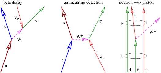
____________________________
In 1979 Sheldon Glashow, Abdus Salam, and Steven Weinberg won the Nobel Prize for their electroweak theory, which unites the electromagnetic and weak interactions. Unlike the strong and electromagnetic forces, the intermediary particles of the weak interaction, the W+, the W-, and the Z0 have rather large masses. In particular, the rest energy of the W± is 81 GeV while that of the Z0 is 92 GeV. Electroweak theory considers electromagnetism and the weak interactions to be different aspects of the same force. A key aspect of the theory is the explanation of why three out of four of the intermediary particles of the electroweak force are massive. (The photon is the massless one.) Unfortunately, the details of why this is so are highly technical, so we cannot delve into this subject here. We only note that the explanation requires the existence of a massive spin zero boson called the Higgs particle. As noted previously, this particle has been discovered recently.
The weak force has certain bizarre properties not shared by the other forces of nature:
The prototypical weak interaction is the decay of the neutron into a proton, an electron, and an antineutrino. This decay is energetically possible because the neutron is slightly more massive than the proton and is illustrated in the left panel of figure 20.3. Note that this figure is drawn as if a neutrino moving backward in time absorbs a W- particle, with a resulting electron exiting the reaction forward in time. However, we know that this is equivalent to an electron and an antineutrino both exiting the reaction forward in time according to the Feynman interpretation of negative energy states.
The weak interaction is called “weak” because it appears to be so in commonly observed processes. For instance, the range of a relativistic electron in ordinary matter is of order centimeters to meters. This is because the electromagnetic force between the charge of the electron and the charges on atomic nuclei are strong enough to rapidly cause the energy of the electron to be dissipated. However, the range in matter of a neutrino produced by beta decay is many orders of magnitude greater than that of an electron. This is not because the weak force is intrinsically weak — the value of the “fine structure constant” for the weak force is
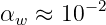 | (20.2) |
according to the standard model, and is actually larger than α for electromagnetism.
The real reason for the apparent weakness of the weak force is the large mass of the intermediary particles. As we have seen, large mass translates into short range for a virtual particle at low momentum transfers. This short range is what causes the weak force to appear weak for momentum transfers much less than the masses of the W and Z particles, i. e., for q ≪ 100 GeV. For leptons and quarks with energies E ≫ 100 GeV, the weak force acts with much the same strength as the electromagnetic force.
| Generation | Leptons | Quarks |
| 1 | electron | down |
| electron neutrino | up | |
| 2 | muon | strange |
| mu neutrino | charm | |
| 3 | tau | bottom |
| tau neutrino | top | |
____________________________
The standard model is a great achievement, but it leaves a number of questions unanswered. As table 20.4 shows, nature seems to have produced more particles than are needed to construct the universe. Virtually everything we know of is composed of electrons, electron neutrinos, up quarks, and down quarks. These four particles seem to fall naturally together in a family or generation. Why then are there apparently unneeded additional generations? What role do muons, taus, and the exotic quark forms play in the universe?
Another question concerns the dichotomy between leptons and quarks. Electrons and electron neutrinos can be converted into each other by weak interactions, as can up and down quarks. Why then can’t quarks be converted into leptons and vice versa?
In the standard model, electromagnetic and weak forces are truly united as aspects of a single phenomenon. However, quantum chromodynamics stands more on its own. One could imagine further advances that would show that the electroweak and strong forces were in fact different aspects of the same phenomenon. This could be characterized as a grand unification of the forces of nature.
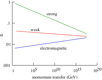
____________________________
As previously noted, the strong force coupling constant, αs, gets smaller with increasing momentum transfer. It turns out that the weak coupling constant, αw, exhibits similar behavior, while the electromagnetic coupling constant, the fine structure constant α, becomes stronger at higher energies. This behavior is illustrated in figure 20.4, though it is based on data only up to about 103 GeV/c. Figure 20.4 is thus largely speculative. However, if the observed trends do continue to very high momentum transfers, this would be evidence in favor of grand unification.
A number of speculative grand unification theories have been proposed. Most such theories view leptons and quarks as being different states of the same particle and also predict that leptons can turn into quarks and vice versa, albeit at very low rates. One of the consequences of such theories is that the proton would be an unstable particle, but with a very long lifetime, of order 1030 yr. Experiments have been done to detect the decay of the proton, but so far without success. These experiments are sufficient to rule out some but not all of the proposed grand unification theories.
One task that would not be accomplished by grand unification is the incorporation of gravity into a common framework with the strong, weak and electromagnetic forces. Creation of a satisfactory quantum theory of gravity has been a very difficult problem and is unsolved to this day, though many people are working on it.
Note: Z = 16 is sulfur and Z = 18 is argon.
Reminder: p = u,u,d; π- = u,d.
Atomic nuclei are composite particles made up of protons and neutrons. These two particles are collectively known as nucleons. In order to better understand atomic nuclei, we first make an analogy with molecules. We then investigate the binding energies of atomic nuclei. This information is central to the subjects of radioactive decay as well as nuclear fission and fusion.
Molecules are bound states of two or more atoms. In chemistry we identify several modes of molecular binding, e. g., covalent and ionic bonds, the hydrogen bond, and binding at low temperatures due to the van der Waal’s force. All of these bonds involve electromagnetic forces, but all (except arguably the ionic bond) are relatively subtle residual forces between atoms that are electrically neutral. The ways in which atoms form molecules are therefore complex and resistent to accurate calculation.
Atomic nuclei are the nuclear equivalent of molecules, in that they are bound states of nucleons, which are themselves “uncharged” composite particles. The charge we refer to here is not the electric charge (nuclei do of course possess this!), but the strong or color charge. As we discovered in the previous chapter, nucleons are color-neutral combinations of quarks. Thus, the “strong” forces between nucleons are subtle residuals of inter-quark forces. This is reflected in the binding energies; quark-quark binding energies are on the order of the rest energies of the quarks themselves. However, nuclear binding energies are typically of order 10 MeV per nucleon, or about 1% of the rest energy of a nucleon.
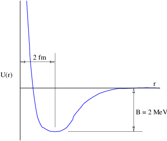
____________________________
The residual nature of nuclear forces makes them complex and difficult to calculate from our basic knowledge of quantum chromodynamics for the same reasons that intermolecular forces are difficult to calculate. An empirical approach is thus needed in order to understand their effects.
In contrast to molecules and atomic nuclei, atoms are relatively easy to understand. This is true for two reasons: (1) Electrons appear to be truly fundamental point particles. (2) Though the atomic nucleus itself is a very complex system, little of this complexity spills over into atomic calculations, because on the atomic scale the nucleus is very nearly a point particle. Thus, both main ingredients in atoms are “simple” from the point of view of atomic calculations.
The above result is true because by some accident of nature, the mass of the electron is so much less than the masses of quarks. It would be interesting to speculate what atomic theory would be like if this weren’t true — there would be no scale separation between the atomic and nuclear scales, and the world would be a very different place!
It is impossible to specify an accurate inter-nucleon force valid under all circumstances, but figure 21.1 gives an approximate representation of the potential energy associated with the strong force as the function of nucleon separation. The binding energy is of order 2 MeV, with an attractive force for separations greater than about 2 × 10-15 m and an intense repulsive force for smaller separations. At large distances the potential energy decays exponentially with distance rather than according to the r-1 law of the Coulomb potential.
The short range of the inter-nuclear force means that atomic nuclei can be thought of as conglomerations of “sticky billiard balls”. The nuclear force is essentially a contact force and each nucleon simply binds to all its nearest neighbors. When nucleons are close-packed, the binding energy per nucleon due to the strong force is simply the number of nearest neighbors for each nucleon, multiplied by the binding energy per nucleon pair, divided by 2. The factor of 1∕2 accounts for the fact that each nuclear bond is shared by two nucleons.
Several other effects need to be accounted for in the nucleus. The nucleons on the surface of the nucleus do not have as many bonds as nucleons in the interior. Thus, to compute the nuclear binding energy of a nucleus with a finite number of nucleons, a correction must be made for this effect. This contributes negatively to the nuclear binding energy in proportion to the surface area of the nucleus, which scales as the number of nucleons to the two-thirds power.
In addition to the nuclear force, the repulsive electrostatic force between protons needs to be accounted for. Since the electrostatic force is a long range force, the (negative) contribution to the binding energy of the nucleus goes as the square of the number of protons divided by the radius of the nucleus. The latter goes as the cube root of the number of nucleons.
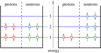
____________________________
The Pauli exclusion principle operates in nuclei so as to favor equal numbers of protons and neutrons. This effect is illustrated in figure 21.2. If a proton is converted into a neutron in a nucleus in which equal numbers of the two particles occur, then the exclusion principle forces these nucleons to move to a higher energy level than they previously occupied. The binding energy of the nucleus is correspondingly decreased. This effect opposes the weaker, repulsive Coulomb potential that occurs when there are more neutrons and fewer protons.
The net result of all these effects is a nuclear binding energy equation with four terms representing the four above-mentioned effects:
 | (21.1) |
where Z is the atomic number or the number of protons, N is the number of neutrons, and A = Z + N is the atomic mass number, or number of nucleons. Equation (21.1) represents the binding energy of the entire nucleus. The binding energy per nucleon is just B∕A.
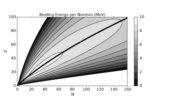
____________________________
Fitting equation 21.1 to observed binding energies in nuclei yields the following values for the coefficients of the above equation: av ≈ 16 MeV, as ≈ 17 MeV, ac ≈ 0.70 MeV, and aa ≈ 23 MeV. A contour plot of binding energy per nucleon, B∕A, is shown in figure 21.3. We note that this equation doesn’t work well for nuclei with only a few nucleons. For instance, the helium nucleus with A = 4 is more stable than the lithium nucleus with A = 6, and there is no stable nucleus at all with A = 5.
Part of the reason for the problem at small A is that even numbers of protons and neutrons tend to bind more strongly together than nuclei containing odd numbers of either. This is because pairs of protons or neutrons with opposite spins fully occupy nuclear states while an odd nucleon occupies a state by itself with energy greater than that of all the other occupied states. This behavior can be approximately accounted for by adding the term ap∕A1∕2 to equation (21.1), where ap = 12 MeV if N and Z are both even, ap = 0 if either N or Z is odd, and ap = -12 MeV if both are odd. We leave this term off even though it is sometimes quite important, in order to make equation (21.1) a smooth function of Z and A and thus representative of the general trend of binding energy.
For a given value of A, it is easy to demonstrate that the maximum nuclear binding energy in equation (21.1) occurs when
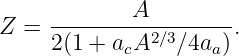 | (21.2) |
This formula confirms the trend seen in figure 21.3 that the most stable nuclear configuration contains an increasing fraction of neutrons as A increases. The function Z(N) given by equation (21.2) and illustrated by the curve starting near the origin in figure 21.3 defines the line of stability for atomic nuclei.
Figure 21.4 shows the binding energy per nucleon as a function of nucleon number A along the line of stability. The rapid increase in binding energy for small A reflects the decreasing surface effect as the number of nucleons increases. The subsequent decrease is a result of the combined effects of Coulomb repulsion of protons and the Pauli exclusion principle. Notice that the maximum binding energy per nucleon occurs near A = 60.
The chemical properties of the atom associated with an atomic nucleus are determined by the number of protons, Z, in the nucleus. In many cases there exists more than one stable or long-lived nucleus with a given value of Z. These nuclei differ in their neutron number, N. Nuclei with the same Z and differing N are called isotopes of the element defined by the specified value of Z. For instance, there are three isotopes of the element hydrogen, normal hydrogen, deuterium, and tritium, with zero, one, and two neutrons respectively.
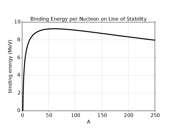
____________________________
Radioactive decay is the emission of some particle from an atomic nucleus, accompanied by a change of state or type of the nucleus, depending on the type of radioactivity.
Gamma rays or photons are emitted when a nucleus decays from an excited state to its ground state. No transformation of the nuclear type occurs. Photons are often emitted when some other form of radioactive decay leaves the resulting nucleus in an excited state.
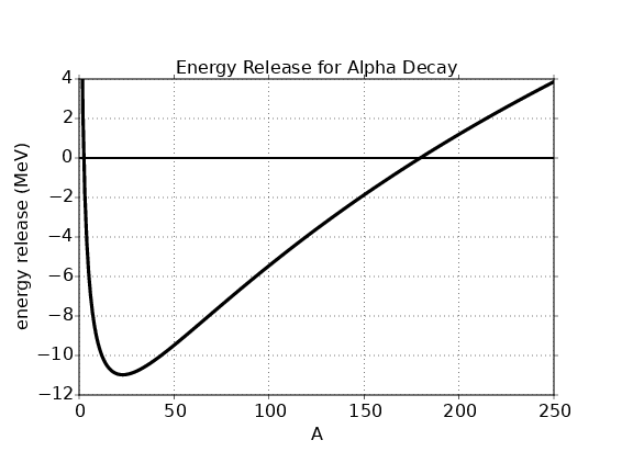
____________________________
Beta minus decay is the conversion of a neutron into a proton, an electron, and an electron antineutrino. This and the inverse reaction, beta plus decay, or conversion of a proton into a neutron, a positron, and an electron neutrino, were described in chapter 18. These processes occur in the nucleons contained in nuclei when they are energetically possible.
Alpha particle emission occurs in heavy elements where it is energetically possible. Since an alpha particle is just a helium 4 nucleus containing two protons and two neutrons, the values of Z and N of the emitting nucleus are each reduced by two.
The rest energy of a nucleus (ignoring atomic effects) is just the sum of the rest energies of all the nucleons minus the total binding energy for the nucleus:
 | (21.3) |
where Mpc2 = 938.280 MeV is the rest energy of the proton and M nc2 = 939.573 MeV is the rest energy of the neutron.
Energy conservation requires that
 | (21.4) |
for the alpha decay of a nucleus. If Q > 0, then the decay is energetically possible. The excess energy, Q, goes into kinetic energy of the new nucleus and the alpha particle, mainly the latter. Substitution of equation (21.3) into equation (21.4) yields
 | (21.5) |
The binding energy of the alpha particle is not accurately represented by equation (21.1), but is known to be about B(2, 4) = 28.3 MeV. On the other hand, the heavy elements are generally well represented by equation (21.1). The curve of Q versus A is plotted in figure 21.5, and it shows that alpha decay for nuclei along the line of stability is energetically impossible (i. e., Q < 0) for nuclei with A less than about 175.
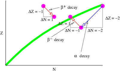
____________________________
Figure 21.6 shows schematically how alpha and beta decay transform atomic nuclei in the N-Z plane. As previously indicated, alpha decay decreases both Z and N by two. Ordinary beta decay (i. e., n → p+ + e- + ν e) decreases N by one and increases Z by one. This is sometimes called β- decay since it produces an electron with negative charge. Though the proton in isolation is stable, the energetics of atomic nuclei are such that a nucleus with a higher proton-neutron ratio than specified by the line of stability can sometimes release energy by the reaction p+ → n + e+ + ν e. This is called β+ decay since it produces a positively charged positron.
Certain isotopes of very heavy elements are at the head of a chain of radioactive decays. This chain consists of a combination of alpha decays interspersed with β- decays. The latter are needed because the alpha decays create nuclei with too low a ratio of protons to neutrons relative to the line of stability, as illustrated in figure 21.6. The beta decays push the chain back toward this line. An example of a chain is one that starts with the element thorium (Z = 90, A = 232) and ends with lead (Z = 82, A = 208). Radioactive decay thus accomplishes what medieval alchemists tried, but failed, to do: transmute elements from one type into another. Unfortunately, no radioactive chain ends at the element gold!
Radioactive decay is governed by a simple law, namely that the rate at which nuclei decay is proportional to the number of remaining nuclei. In mathematical terms, this is expressed as follows:
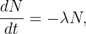 | (21.6) |
where N(t) is the number of remaining nuclei at time t and λ is called the decay rate. This differential equation has the solution
 | (21.7) |
which shows that the number of nuclei decreases exponentially with time.
The half-life, t1∕2 of a certain nuclear type, is the time required for half the nuclei to decay. Setting N(t1∕2) = N(0)∕2, we find that
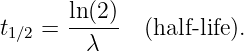 | (21.8) |
The nature of exponential decay means that half the particles are left after one half-life, a quarter after two half-lives, an eighth after three half-lives, etc. The actual value of λ, and hence t1∕2, depends on the character of the nucleus in question, with half-lives ranging from a small fraction of a second to many billions of years.
From figure 21.4 it is clear that atomic nuclei with A < 60 can combine to form more tightly bound nuclei and in so doing release energy. This is called nuclear fusion and it is the process that powers stars.
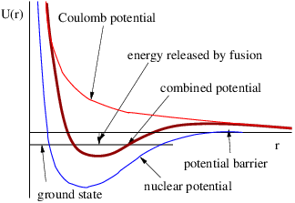
____________________________
It is not easy to fuse two nuclei. As figure 21.7 shows, the nuclear force, which is attractive but short in range, and the Coulomb force, which is repulsive, combine to create a potential barrier that must be surmounted in order to release energy from fusion. Nuclei must therefore somehow attain large kinetic energy for fusion to take place. We shall discover later that temperature is a measure of the translational kinetic energy of atoms and nuclei. Therefore, one way to create fusion is to heat the appropriate material to a very high temperature. The interiors of ordinary stars are hot enough to fuse hydrogen into helium. Somewhat hotter stars can create slightly heavier elements. However, we believe that only the interior of a type of exploding star called a supernova is hot enough to create the heavy elements we find in the universe. Thus, the iron in your automobile engine and the copper in your electrical wiring were created in some of the most spectacular explosions in the universe!
| Nucleus | Z | A | B (MeV) |
| deuterium | 1 | 2 | 2.22 |
| tritium | 1 | 3 | 8.48 |
| helium-3 | 2 | 3 | 7.72 |
| helium-4 | 2 | 4 | 28.30 |
| lithium-6 | 3 | 6 | 32.00 |
| lithium-7 | 3 | 7 | 39.25 |
____________________________
In computing energy balances for light nuclei, it is important to use exact values of binding energies, not the approximate values obtained from the binding energy formula given by equation (21.1), as the values given by this equation for small A can be off by a large amount. Sample values for such nuclei are given in table 21.1.
It is possible for a heavy nucleus such as uranium, with atomic number and atomic mass number (Z,A) to spontaneously fission or split into two lighter nuclei with (Z′,A′) and (Z - Z′,A - A′) if there is a net energy release from this process:
 | (21.9) |
An energy of order 160 MeV per nucleus can be released by causing uranium (Z = 92) or plutonium (Z = 94) to fission.
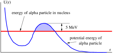
____________________________
Even if Q > 0, spontaneous fission generally occurs at a very slow rate. This is because a potential energy barrier of order 5 MeV typically must be overcome for this split to occur. Barrier penetration allows fission to occur spontaneously in the absence of the energy needed to overcome this barrier, as illustrated in figure 21.8, but is generally a slow process. Alpha decay is an example of spontaneous fission of a heavy nucleus by barrier penetration in which Z′ = 2 and A′ = 4.
If a heavy nucleus collides with an energetic particle such as a neutron, photon, or alpha particle, it can be induced to fission if the energy transferred to the nucleus exceeds the approximate 5 MeV needed to breach the potential barrier.
If the heavy nucleus has an odd number of neutrons, another way for fission to occur is for the nucleus to capture a slow neutron, i. e., one with energy much less than the 5 MeV needed to directly overcome the potential barrier. In this case neutron capture actually converts the nucleus from atomic number and mass (Z,A) to atomic number and mass (Z,A + 1).
The binding energy per nucleon of a nucleus with an even number of neutrons is greater than the binding energy per nucleon of one with an odd number, since in the former case all neutron spins are paired. Thus, if the initial nucleus has an odd number of neutrons, the capture of a slow neutron makes it more tightly bound than if the initial nucleus has an even number of neutrons. If the difference in binding energy between the initial nucleus and the nucleus modified by neutron capture exceeds the 5 MeV needed to overcome the potential barrier for spontaneous fission, then energy conservation leaves the new nucleus in a sufficiently high excited state that it instantly fissions. Examples of nuclei subject to fission by slow neutron absorption are uranium 235 and plutonium 239. Note that both have odd numbers of neutrons. In contrast, uranium 238 has an even number of neutrons and slow neutron bombardment does not cause fission.
Human beings have long had an intuitive understanding of heat and temperature from personal experience. We sense that different things often have different temperatures and we know that objects tend to acquire the same temperature after being placed in physical contact for some time. We view this equilibration process as a flow of “heat” (whatever that is) from the warmer body to the cooler body.
A need for a more precise understanding of the behavior of heat and temperature was felt with the development of the steam engine. The science of thermodynamics arose out of this need. Thermodynamics was developed before we understood the atomic nature of matter. More recently the ideas of thermodynamics were related to mechanical processes happening on the atomic scale. Today we understand the phenomena of heat and temperature to be aspects of the collective mechanical behavior of large numbers of atoms and molecules.
We measure temperature by a variety of means. The most primitive measurement is direct sensing by the human body. We immediately discern whether something we touch is hot or cold relative to our own body. Furthermore, we can detect a hot stove from a distance by the feeling of warmth on our skin. In the case of direct contact, heat is transferred to our hand by conduction, whereas in the latter case the transfer takes place by thermal radiation. Our body considers something to be hot if heat is transferred from the object to our body, whereas it is perceived as being cold if the transfer of heat is from our body to the object.
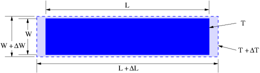
____________________________
A more objective measure of temperature is obtained by using the fact that ordinary material objects expand when they become warmer and contract when they cool. Empirically it is found that the fractional change in the length of a solid body, ΔL∕L, is related to the change in temperature ΔT, as illustrated in figure 22.1:
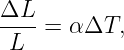 | (22.1) |
where α is called the linear coefficient of thermal expansion.
For liquids the fractional change in volume, ΔV∕V , is easier to relate to the change in temperature than the fractional change in linear dimension:
 | (22.2) |
where β is the volume coefficient of thermal expansion. The quantities α and β depend on the material properties and on the temperature scale being used. The ordinary thermometer is based on the thermal expansion of a liquid such as mercury.
The most commonly used temperature scales in science are the Celsius and Kelvin scales. Roughly speaking, water freezes at 0∘ C and it boils (at sea level) at 100∘ C. More precise definition of the Celsius scale depends on a detailed understanding of the phase changes of water, which we won’t develop here.
There is a limit to how cold something can be. The Kelvin scale is designed to go to zero at this minimum temperature. The relationship between the Kelvin temperature T and the Celsius temperature TC is
 | (22.3) |
Thus, water freezes at about 273 K and boils at about 373 K. (Notice that the little circle or degree sign is used for Celsius temperatures but not Kelvin temperatures.) Unless otherwise noted, we will use the Kelvin scale. Table 22.1 gives values of α and β for some common materials.
| Material | α (K-1) | β (K-1) |
| steel | 12 × 10-6 | — |
| copper | 16 × 10-6 | — |
| aluminum | 23 × 10-6 | — |
| invar | 0.7 × 10⁻⁶ | — |
| glass | 9 × 10⁻⁶ | — |
| lead | 29 × 10-6 | — |
| methyl alcohol | — | 1.22 × 10⁻³ |
| glycerine | — | 0.53 × 10⁻³ |
| mercury | — | 0.182 × 10⁻³ |
| water (15∘ C) | — | 0.15 × 10⁻³ |
| water (35∘ C) | — | 0.35 × 10⁻³ |
| water (90∘ C) | — | 0.70 × 10⁻³ |
____________________________
Accurate temperature measurements depend in practice on a knowledge of the properties of materials under temperature changes. However, we shall find later that the concept of temperature can be defined in a way that is completely independent of material properties.
Two types of experiments suggest that heating is a form of energy transfer. First of all, on the macroscopic or everyday scale of things, there are forces that are apparently nonconservative. This is in marked contrast to the microscopic world, where forces are either conservative (gravity, electrostatics), don’t change a particle’s energy (magnetic force), or convert energy from one known form to another (non-static electric forces). With these fundamental forces all energy is accounted for — it is neither created or destroyed.
In contrast, macroscopic energy routinely disappears in the everyday world. Cars once set in motion don’t continue in motion forever on a level road once the engine is stopped; a soccer ball once kicked eventually comes to rest; electrical energy powering a light bulb appears to be lost. Careful measurements show that whenever this type of energy loss is found, heating occurs. Since we believe that macroscopic forces are really just large scale manifestations of fundamental microscopic forces, we do not believe that energy really disappears as a result of these forces — it must simply be converted from a form visible to us into an invisible form. We now know that such forces convert macroscopic energy to internal energy, a form of energy that is just the kinetic and potential energy of atomic and molecular motions. Thus, the apparent disappearance of macroscopic energy is just a consequence of the conversion of this energy into microscopic form.
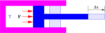
____________________________
The second type of experiment that suggests that heating converts macroscopic energy to internal energy is one in which this energy is converted back to macroscopic form. An example of this process is illustrated in figure 22.2. As the piston moves out of the cylinder under the force exerted on it by the gas, work is done that can be stored or used by, say, compressing a spring or running an electric generator. As the piston moves out, the gas in the cylinder decreases in temperature, which indicates that the gas is losing microscopic energy.
Conversion of macroscopic energy to microscopic kinetic energy thus tends to raise the temperature, while the reverse conversion lowers it. It is easy to show experimentally that the amount of heating needed to change the temperature of a body by some amount is proportional to the amount of matter in the body. Thus, it is natural to write
 | (22.4) |
where M is the mass of material, ΔQ is the amount of energy transferred to the material, and ΔT is the change of the material’s temperature. The quantity C is called the specific heat of the material in question and is the amount of heating needed to raise the temperature of a unit mass of material by one degree. C varies with the type of material. Values for common materials are given in table 22.2.
| Material | C (J kg-1 K-1) |
| brass | 385 |
| glass | 669 |
| ice | 2092 |
| steel | 448 |
| methyl alcohol | 2510 |
| glycerine | 2427 |
| water | 4184 |
____________________________
We now address some questions of terminology. The use of the terms “heat” and “quantity of heat” to indicate the amount of microscopic kinetic energy inhabiting a body has long been out of favor due to their association with the discredited “caloric” theory of heat. Instead, we use the term internal energy to describe the amount of microscopic energy in a body. The word heat is most correctly used only as a verb, e. g., “to heat the house”. Heat thus represents the transfer of internal energy from one body to another or conversion of some other form of energy to internal energy. Taking into account these definitions, we can express the idea of energy conservation in some material body by the equation
 | (22.5) |
where ΔE is the change in internal energy resulting from the addition of heat ΔQ to the body and the work ΔW done by the body on the outside world. This equation expresses the first law of thermodynamics. Note that the sign conventions are inconsistent as to the direction of energy flow. However, these conventions result from thinking about heat engines, i. e., machines that take in heat and put out macroscopic work. Examples of heat engines are steam engines, coal and nuclear power plants, the engine in your automobile, and the engines on jet aircraft.
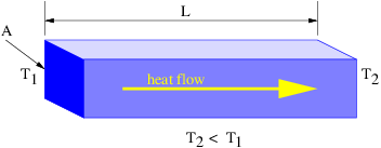
____________________________
As noted earlier, internal energy may be transferred through a material from higher to lower temperature by a process known as heat conduction. The rate at which internal energy is transferred through a material body is known empirically to be proportional to the temperature difference across the body. For a rectangular body, the rate of transfer is also known to scale in proportion to the cross sectional area of the body perpendicular to the temperature gradient and to scale inversely with the distance over which the temperature difference exists. This is known as the law of heat conduction and is expressed in the following mathematical form:
 | (22.6) |
where Fheat is the internal energy per unit time flowing down the temperature gradient, A is the cross sectional area of the body normal to the internal energy flow direction, L is the length of the body in the direction of heat flow, ΔT is the temperature difference along its length, and κ is a constant characteristic of the material known as the thermal conductivity. The geometry is illustrated in figure 22.3 and the thermal conductivities of common materials are shown in table 22.3.
| Material | κ (W m-1 K-1) |
| brass | 109 |
| brick | 0.50 |
| concrete | 1.05 |
| ice | 2.2 |
| paper | 0.050 |
| steel | 46 |
____________________________
Energy can also be transmitted though empty space by thermal radiation. This is nothing more than photons with a mixture of frequencies near a frequency ωthermal that is a function only of the temperature T of the body that is emitting them:
 | (22.7) |
where the constant K = 3.67 × 10¹¹ s-1 K-1. The amount of thermal energy per unit area per unit time emitted by a material surface is called the flux of radiation and is given by Stefan’s law:
 | (22.8) |
where σ = 5.67 × 10⁻⁸ W m-2 K-4 is the Stefan-Boltzmann constant and ε is the emissivity of the material surface. The emissivity lies in the range 0 ≤ ε ≤ 1 and depends on the type of material and the temperature of the surface.
Surfaces that emit thermal radiation at a particular frequency can also reflect radiation at that frequency. If JI is the flux of radiation incident on the surface, then the reflected radiation is just
 | (22.9) |
and the balance of the radiation is absorbed by the surface:
 | (22.10) |
Thus, high thermal emissivity goes along with high absorbed fraction and vice versa. A little thought indicates why this has to be so. If the emissivity were high and the absorption were low, then the object would spontaneously cool relative to its environment. If the reverse were true, it would spontaneously warm up. Thus, the universally observed behavior that internal energy flows from higher to lower temperatures would be violated.
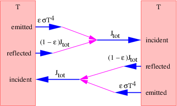
____________________________
Imagine two surfaces of equal temperature T facing each other. The radiation emitted by one surface is partially absorbed and partially reflected from the other surface, as illustrated in figure 22.4. The total radiative flux, Jtot, coming from each surface is the sum of the reflected radiation originating from the other surface, (1 - ε)Jtot, and the emitted thermal radiation, εσT4. Thus,
 | (22.11) |
Solving for Jtot, we find that
 | (22.12) |
Note that the total radiation originating from each surface, Jtot, is independent of the emissivity of the surfaces and depends only on the temperature. This radiative flux is called the black body flux. We give it the special name JBB. Because it no longer depends on ε, it is independent of the character of the material making up the emitting surfaces. Different materials result in different fractions of thermal and reflected radiation, but the sum is always equal to the black body flux if both surfaces are at the same temperature. Planck’s arguments that led to the energy-frequency relationship of quantum mechanics, E = ℏω, came from his attempt to explain black body radiation. The laws of black body radiation presented here can be derived from quantum mechanics.
In this section we consider the quantitative forms of non-conservative forces on the macroscopic level. We first examine the frictional force between two solid bodies and then consider viscosity in liquids.
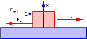
____________________________
The frictional force Fk between two solid objects in contact obeys an empirical law.1 If the two objects are sliding over each other, the frictional force on each object acts so as to oppose the relative motion of the two objects. (See figure 22.5.) The frictional force is proportional to the normal force N pressing the objects together:
 | (22.13) |
The dimensionless quantity μk is called the coefficient of kinetic friction. This quantity is different for different pairs of materials rubbing together. It is typically of order one, but may be much less for particularly slippery materials.
Equation (22.13) is only valid if the two objects are moving relative to each other. If they are not in relative motion, but if some other force is being exerted on one of them, a static frictional force Fs will precisely counteract this force so as to result in zero net force on the object. However, the static frictional force will keep the bodies from slipping only up to some limit defined by
 | (22.14) |
where μs is the coefficient of static friction. Generally we find that μs > μk, so gradually increasing the external force on an object in static frictional contact with another object will cause it to suddenly break loose and accelerate when the maximum sustainable static frictional force is exceeded. Once the object is in motion, a lesser external force is needed to keep it moving at a constant velocity.
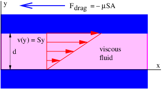
____________________________
If two objects are not in physical contact but are separated by a thin layer of fluid (i. e., a liquid or a gas), there is still a frictional or viscous drag force between the two objects, but its behavior is different. Figure 22.6 tells the story: The viscous drag force in this case is
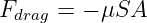 | (22.15) |
where S = vp∕d is the shear in the fluid, A is the area of the plates, and μ is the viscosity of the fluid. (Don’t confuse this parameter with the static and dynamic coefficients of friction!) The parameter vp is the velocity of the top plate with respect to the bottom plate and d is the separation between the plates.
Viscosity has the dimensions mass per length per time. The most common unit of viscosity is the Poise: 1 Poise = 1 g cm-1 s-1. The viscosity of water varies from 0.0179 Poise at 0∘ C to 0.0100 Poise at 20∘ C to 0.0028 Poise at 100∘ C. The viscosity of water thus decreases with increasing temperature, which is typical of liquids. In contrast, the viscosity of a gas is independent of the density of the gas and is proportional to the square root of its absolute temperature. The viscosity of a gas thus increases with temperature, in contrast to the viscosity of a liquid. For air at 20∘ C, the viscosity is 1.81 × 10⁻⁴ Poise.
Thin layers of oil between moving parts are commonly used in machinery to reduce friction, since the resulting viscous drag is generally much less than the corresponding kinetic friction that would occur if the parts were in direct contact. The ways in which the layer of oil is maintained between moving parts are fascinating, but beyond the scope of this course.
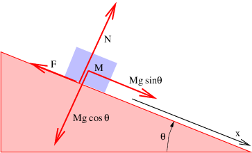
_____________________________________
So far we have taken a purely empirical view of the properties of systems composed of many atoms. However, as previously noted, it is possible to understand such systems using the underlying principles of mechanics. The resulting branch of physics is called statistical mechanics. J. Willard Gibbs, a late 19th century American physicist from Yale University, almost single-handedly laid the groundwork for the modern form of this subject. Interestingly, the quantum mechanical version of statistical mechanics is much easier to understand than the version that Gibbs developed, which is based on classical mechanics. It also gives correct answers where the Gibbs version fails.
A system of many atoms has many quantum mechanical states in which it can exist. Think of, say, a brick. The atoms in a brick are not stationary; they are in a continual flurry of vibration at ordinary temperatures. The kinetic and potential energies associated with these vibrations constitute the internal energy of the brick.
Though the details of each state are unimportant, the number of states turns out to be a crucial piece of information. To understand why this is so, let us imagine two bricks identical in composition and mass. Brick A has internal energy between E and E + ΔE and brick B has energy between 0 and ΔE. Think of ΔE as the uncertainty in the energy of the bricks; we can only observe a brick for a finite amount of time Δt, so the uncertainty principle asserts that the uncertainty in the energy is ΔE ≈ℏ∕Δt.
The brick is a complex system consisting of many atoms, so in general there are many possible quantum mechanical states available to brick A in the energy range E to E + ΔE. It turns out, for reasons that we will see later, that significantly fewer states are available to brick B in the energy range 0 to ΔE than are available to brick A.
Roughly speaking, the larger the internal energy of an object per unit mass, the higher is its temperature. Thus, we infer that brick A has a much higher temperature than brick B. What happens when we bring the two bricks into thermal contact? Our experience tells us that heat (i. e., internal energy) immediately starts to flow from one brick to the other, ultimately resulting in an equilibrium state in which the temperature is the same in the two bricks.
We explain this process as follows. Statistical mechanics hypothesizes that any system of atoms (such as a brick) is free to roam through all quantum mechanical states that are energetically available to it. In fact, this roaming is assumed to be continually taking place. Given this picture and the assumption that the roaming between states is completely random, one would expect equal probabilities for finding the system in any particular state.
Of course, this probability argument assumes that we don’t know anything about the initial state of the system. If the system is known to be in some particular state at time t = 0, then it will take some time for the system to evolve in such a way that it has “forgotten” the initial state. During this interval our knowledge of the initial state and the quantum mechanical dynamics of the system can be used (in principle) to follow the evolution of the system. Eventually the uncertainty in our initial knowledge of the system catches up with us and we cannot predict the future evolution of the system beyond this point. The brick develops “amnesia” and its probability of being in any of the energetically allowed states is then uniform.
Something like this happens to the two bricks if they are brought into thermal contact. Initially brick A has virtually all of the energy and brick B has only a tiny amount. When the bricks are brought into contact, they eventually can be treated as a single brick of twice the size. However, it takes time for the new, larger brick to evolve to the point where it has forgotten the fact that it started out as two separate bricks at different temperatures. In this interval the temperature of brick A is decreasing while the temperature of brick B is increasing as a result of internal energy flowing from one to the other. This evolution continues until equilibrium is reached.
Even though the combined brick has forgotten its initial state, there is a small chance that it will return to this state, since the probability of finding the brick in any state, including the original one, is non-zero. Thus, according to the postulates of statistical mechanics, one might suddenly find the brick again in a state in which virtually all of the internal energy is concentrated in former brick A. Actually, the issue is slightly more complicated than this. Brick A actually had many states available to it before being brought together with brick B. Thus, a more interesting problem is to find the probability of the system suddenly finding itself in any of the states in which (virtually) all of the energy is concentrated in former brick A. Given the randomness assumption of statistical mechanics, this probability is simply the number of states that correspond to all of the energy being in brick A, divided by the total number of states available to the combined brick. Computing this number is the task we set for ourselves.
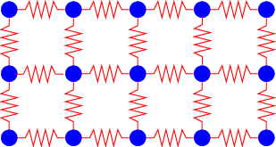
____________________________
In this section we demonstrate the above assertions by making a crude model of the quantum mechanical states of a brick. We approximate the atoms of the brick as a collection of harmonic oscillators, three oscillators per atom, since each atom can oscillate in three dimensions under the influence of interatomic forces (see figure 23.1). For simplicity we assume that all of the oscillators have the same classical oscillation frequency, ω0, so that the energy of each oscillator is given by
 | (23.1) |
as reported in chapter 12. This assumption is a rather poor approximation to the behavior of a solid body when the total amount of internal energy is so small that many of the harmonic oscillators are in their ground state. However, it is adequate for situations in which the energy per oscillator is several times the ground state oscillator energy.
We further assume that each oscillator is weakly coupled to its neighbor. This allows a slow transfer of energy between oscillators without appreciably affecting the energy levels of each oscillator.
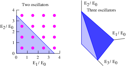
____________________________
The next step is to calculate the number of states of a system of harmonic
oscillators for which the total energy is less than some maximum value E. This
calculation is easy for a system consisting of a single oscillator. From equation
(23.1) we infer that the number of states,  , of one oscillator with energy less
than E is
, of one oscillator with energy less
than E is
 | (23.2) |
since the states are evenly spaced in energy with spacing E0.
The calculation for a system of two oscillators is slightly more complicated. The dots in the left panel of figure 23.2 show the states available to a two oscillator system. Each dot corresponds to a unique pair of values of the quantum numbers n1 and n2 for the two oscillators. The total energy of the two oscillators together is Etotal = E1 + E2 = (n1 + n2 + 1)E0.
The line defined by the equation E∕E0 = E1∕E0 + E2∕E0 is illustrated by the hypotenuse of the shaded triangle in the left panel of figure 23.2. The number of states with total energy less than E is obtained by simply counting the dots inside this triangle. An easy way to do this “counting” is to note that there is one dot per unit area in the plot, so that the number of dots approximately equals the area of the triangle:
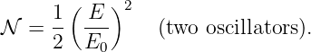 | (23.3) |
For a system of three oscillators the possible states of the system form a cubical grid in a three-dimensional space with axes E1∕E0, E2∕E0, and E3∕E0, as shown in the right panel of figure 23.2. The dots representing the states are omitted for clarity, but one state per unit volume exists in this space. The dark-shaded oblique triangle is the surface of constant total energy E defined by the equation E1∕E0 + E2∕E0 + E3∕E0 = E∕E0, so the volume of the tetrahedron formed by this surface and the coordinate axis planes equals the number of states with energy less than E. This volume is computed as the area of the base of the tetrahedron, (E∕E0)2∕2, times its height, E∕E 0, times 1∕3. We get
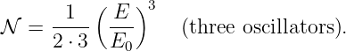 | (23.4) |
There is a pattern here. We infer that there are
 | (23.5) |
states available to N oscillators with total energy less than E. The notation N! is shorthand for 1 ⋅ 2 ⋅ 3…N and is pronounced “N factorial”.
Let us summarize what we have accomplished. (E) is the number of states
of a system of harmonic oscillators, taken together, with total energy less than E.
What we need is an estimate of the number of states between two energy limits,
say E and E + ΔE. This is easily obtained from (E) as follows: (E) is the
number of states with energy less than E, while (E + ΔE) is the number
of states with energy less than E + ΔE. We can obtain the number of
states with energies between E and E + ΔE by subtracting these two
quantities:
 | (23.6) |
For N harmonic oscillators we find that
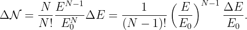 | (23.7) |
| N | Δ (r = 5) | Δ (r = 10) |
| 1 | 1 | 1 |
| 2 | 5 | 10 |
| 3 | 50 | 200 |
| 4 | 563 | 4500 |
| 5 | 6667 | 106667 |
| 6 | 81381 | 2604167 |
| 7 | 1012500 | 64800000 |
| 8 | 12765734 | 1634013889 |
| 9 | 162539683 | 41610158730 |
| 10 | 2085209002 | 1067627008928 |
| 11 | 26911444555 | 27557319223986 |
| 12 | 349006782021 | 714765889577822 |
available to N identical harmonic
oscillators between energies E and E + ΔE, where E = rNE0 and where we
have chosen ΔE = E0. Results are shown for two different values of r.____________________________
Table 23.1 shows the number of states of a system of a small number of harmonic oscillators with energy between E and E + ΔE where we have chosen ΔE = E0. Results are shown for systems up to N = 12 (i. e., “microbricks” with up to 4 atoms, each with 3 modes of oscillation). The quantity r is defined to be the average value of the quantum number n of all the harmonic oscillators in the system; r = E∕(NE0). Thus, rE0 is the average energy per oscillator. Recall that our calculation is only valid if r is appreciably greater than one. The number of available states is computed for r = 5 and 10.
We see that a few atoms considered jointly have an astonishingly large number of possible states. For instance, a system of 4 atoms (i. e., 12 oscillators) with r = 5 has about 3.5 × 10¹¹ states. Suppose we now confine this energy to only 2 of the atoms or 6 oscillators. In this case r doubles to a value of 10 since the same amount of internal energy is now spread among half the number of oscillators. Table 23.1 shows that this reduced system has only about 2.6 × 10⁶ states. The probability of having all of the energy of the 4 atom system in these 2 atoms is the ratio of the number of states in the 2 atom case to the total number of possible states of the 4 atom system, or 2.6 × 10⁶∕3.5 × 1011 = 7.4 × 10⁻⁶. This is a rather small number, which means that it is rare to find the system with all internal energy concentrated in two atoms.
We now determine how the number of states available to a system of harmonic
oscillators behaves for a very large number of oscillators such as might be found in
a real brick. Values of Δ become so large in this case that it is useful to
work in terms of the natural logarithm of Δ. For large N we can safely
approximate N - 1 by N. Using the properties of logarithms, we get
 | (23.9) |
Substituting this into equation (23.8), using the fact that N ln(E∕E0) - N ln N = N ln[E∕(NE0)], and rearranging results in
![[ ( -E---) ] ( ΔE--)
ln(ΔN ) = N ln N E + 1 + ln E (N oscillators).
0 0](book2193x.png) | (23.10) |
We now return to the original question, which we state in this form: What
fraction of the states of a brick corresponds to the special situation with all of the
internal energy in half of the brick? A real brick has of order 3 × 1025 atoms or
about N = 1026 oscillators. Half of the brick thus has N′ = 5 × 1025 oscillators. If,
as before, we assume that r = 5 when the internal energy is distributed
throughout the brick, then we have r′ = 10 when all the energy is in half
of the brick. Therefore the logarithm of the total number of available
states is ln(Δ) = N[ln(r) + 1] + ln(ΔE∕E0), while the logarithm of
the number of states available when all the energy is in half of the brick
is ln(Δ′) = N′[ln(r′) + 1] + ln(ΔE∕E0). Putting in the numbers, we
find that the probability of finding all the energy in half of the brick is
![′ ′
ΔN ∕ΔN = exp[ln (ΔN ) - ln (ΔN )]
= exp[N ′ln(r′) + N ′ + ln(ΔE ∕E0 )
- N ln(r) - N - ln (ΔE ∕E0 )]
= exp(- 0.96N ) = exp(- 9.6 × 1025) = 10- 4.2×1025.(23.11)](book2194x.png)
Notice that ΔE, which we haven’t specified, cancels out. This typically happens in the theory when measurable quantities are calculated, and it shows that the actual value of ΔE isn’t important. Furthermore, for very large values of N typical of normal bricks, the term in equation (23.10) containing ΔE is always negligible for any reasonable values of ΔE. We therefore drop it in future calculations.
The variable ln(Δ) is proportional to a quantity that we call the entropy, S.
The actual relationship is
 | (23.12) |
where kB = 1.38 × 10⁻²³ J K-1 is called Boltzmann’s constant. Ludwig Boltzmann was a 19th century Austrian physicist who played a pivotal role in the development of the concept of entropy. The entropy of a brick containing N oscillators is therefore
![[ ( E ) ]
S = N kB ln ----- + 1 (entropy of N oscillators).
N E0](book2196x.png) | (23.13) |
As with the speed of light and Planck’s constant, Boltzmann’s constant is not really needed for a complete development of statistical mechanics. Its only role is to convert entropy and related quantities to everyday units. The conventional dimensions of entropy are thus the same as those of Boltzmann’s constant, or energy divided by temperature. However, more fundamentally, we consider entropy (without Boltzmann’s constant) to be a dimensionless quantity since it is just the logarithm of the number of available states.
What use is entropy? In our example we found that the number of states for the situation in which all of the internal energy of a brick is restricted to half of the brick is much less than the number of states available when no restrictions are put upon the distribution of the same amount of internal energy through the entire brick. Thus, the entropy, which is just proportional to the logarithm of the number of available states, is less in the restricted case than it is in the unrestricted case.
This turns out to be generally true. Any measurable restriction we place on the distribution of internal energy in the brick turns out to result in a much smaller number of available quantum mechanical states and hence a smaller value for the entropy. Once such a restriction is lifted, all possible states become available, and according to the postulates of statistical mechanics the brick eventually evolves to the point where it is roaming randomly through these states. The probability of the brick revisiting the original restricted set of states is so small as to be completely ignorable once it forgets its initial state, because these states form only a miniscule fraction of the states available to the brick. Thus, with a very high degree of certainty, one can say that the entropy of the brick increases when the restriction is lifted.
Strictly speaking, our definition of entropy is only valid after the brick has reached equilibrium, i. e., when the initial state has been forgotten. The entropy during the equilibration period according to our definition is technically undefined.
Our inferences about a brick can be extended to any isolated system, i. e., any system that doesn’t exchange mass or energy with the outside world: The entropy of any isolated system consisting of a large number of atoms will not spontaneously decrease with time. This principle is called the second law of thermodynamics.
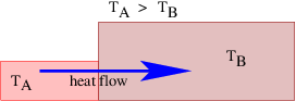
____________________________
Where does the idea of temperature fit into the picture? This concept has come up informally, but we need to give it a precise definition. If two objects at different temperatures are placed in contact with each other, we observe that internal energy flows from the warmer object to the cooler object, as illustrated in figure 23.3.
We wish to see if the role of temperature differences in the flow of internal energy can be related to the ideas developed in the previous section. Let us consider two bricks as before, but possibly of different size, and therefore containing different numbers of harmonic oscillators. Suppose brick A has NA oscillators and energy EA while brick B has NB oscillators and energy EB. The two bricks have entropies
![[ ( E ) ]
SA = kBNA ln ---A-- + 1
NAE0](book2197x.png) | (23.14) |
and
![[ ( E ) ]
SB = kBNB ln ---B-- + 1 .
NBE0](book2198x.png) | (23.15) |
If the two bricks are thermally isolated from each other but are nevertheless considered together as one system, then the total number of states available to this combined system is just the product of the numbers of states available to each brick separately:
 | (23.16) |
To make an analogy, the total number of ways of arranging two coins, each of which may either be heads up or tails up, is 4 = 2 × 2, or heads-heads, heads-tails, tails-heads, and tails-tails. We compute the states of the combined system just as we compute the total number of ways of arranging the coins, i. e., by taking the product of the numbers of states of the individual systems.
Taking the logarithm of Δ and multiplying by Boltzmann’s constant results
in an equation for the combined entropy S of the two bricks:
 | (23.17) |
In other words, the combined entropy of two (or more) isolated systems is just the sum of their individual entropies.
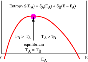
____________________________
We can determine how the total entropy of the two bricks depends on the distribution of energy between them by using equations (23.14) and (23.15). Plotting the sum of the entropies of the two bricks SA(EA) + SB(EB) versus the energy EA of brick A under the constraint that the total energy E = EA + EB is constant yields a curve that typically looks something like figure 23.4. Notice that the total entropy reaches a maximum for some critical value of EA. Since the slope of S(EA) is zero at this point, we can determine the corresponding value of EA by setting the derivative to zero of the total entropy with respect to EA, subject to the condition that the total energy is constant. Under the constraint of constant total energy E, we have dEB∕dEA = d(E - EA)∕dEA = -1, so
 | (23.18) |
(The partial derivatives indicate that parameters besides the energy are held constant while taking the derivative of entropy.) Thus,
 | (23.19) |
at the point of maximum entropy.
Once the equilibrium values of EA and EB are found, we can calculate the total entropy S = SA + SB of two thermally isolated bricks. We now assert that this entropy doesn’t change when two bricks in equilibrium are brought into thermal contact. Why is this so?
The derivative of the entropy of a system with respect to energy turns out to be one over the temperature of the system. Thus, the temperatures of the bricks can be found from
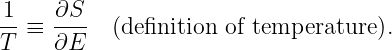 | (23.20) |
The condition for equilibrium (23.19) therefore reduces to 1∕TA = 1∕TB, or TA = TB. This is consistent with observations of the behavior of real systems. Thus, at the equilibrium point the temperatures of the two bricks are the same and bringing them together causes no heat flow to occur. The process of bringing two bricks at the same temperature into thermal contact is thus completely reversible, since separating them leaves each with the same amount of energy it started with.
The temperature of a brick is easily calculated using equation (23.20):
 | (23.21) |
We see that the temperature of a brick is just the average energy per harmonic oscillator in the brick divided by Boltzmann’s constant.
Equation (23.20) provides us with a physical definition of temperature that is independent of specific material properties such as the thermal expansion coefficient of some particular metal. Though different materials have different dependences of entropy on internal energy, the derivative of entropy with respect to energy will be the same for any two materials in thermal equilibrium with each other.
Note that the unit of temperature is the Kelvin degree according to this theory. If we had left off Boltzmann’s constant in the definition of entropy, the dimensions of temperature would be that of energy. Boltzmann’s constant is thus simply a scaling factor that changes temperature to energy just as multiplication by the speed of light converts time to distance.
How can we compute the specific heat of a collection of harmonic oscillators? Starting from the temperature of a brick, as given by equation (23.21), we solve for the brick’s internal energy:
 | (23.22) |
Recall that the specific heat is the heat required per unit mass to increase the temperature of the brick by one degree. For a solid body, essentially all the heat added to the body goes into increasing its internal energy. Thus, if the mass of the brick is M = Nm where m is the mass per oscillator, then the predicted specific heat of the brick is
 | (23.23) |
This formula is in reasonable agreement with measurements when the temperature is high enough so that all the harmonic oscillators are in excited states, i. e., with r > 1. (We equate dQ = dE using the first law of thermodynamics, since no work is being done by the brick.)
Though entropy is formally not defined in a system that is not in thermodynamic equilibrium, one can imagine situations in which elements of a system interact only weakly with other elements. Each element is therefore very close to internal equilibrium, so that the entropy of each element can be defined. However, the elements are not in equilibrium with each other.
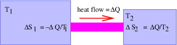
____________________________
Figure 23.5 shows an example of such a situation. Since 1∕T = ∂S∕∂E, one can write
 | (23.24) |
since heat flowing out of region 1 results in a decrease in internal energy ΔE1 = -ΔQ. Likewise, we find that
 | (23.25) |
since the internal energy of region 2 increases by ΔE2 = ΔQ. The total change of entropy of the system is therefore
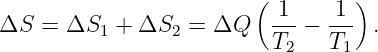 | (23.26) |
From our experience, we know that heat will only flow from region 1 to region 2 if T1 > T2. However, equation (23.26) shows that the net entropy change is positive when this is true. Conversely, if T1 < T2, then the net entropy change would be negative and heat would be flowing spontaneously from lower to higher temperatures. Thus, the statement that heat cannot spontaneously flow from lower to higher temperatures is equivalent to the statement that the entropy of an isolated system must not decrease. An alternative statement of the second law of thermodynamics is therefore heat cannot spontaneously flow from lower to higher temperatures.
If entropy increases in some process, we call it irreversible. Spontaneous heat flow is always irreversible. However, in the limit in which the temperature difference is very small, the entropy increase due to heat flow is also small. Of course, the rate of flow of heat is also quite slow in this case. Nevertheless, this situation forms a useful idealization. In the idealized limit of very small, but nonzero temperature difference, the flow of heat is said to be reversible because the generation of entropy is negligible.
for N harmonic
oscillators.) From this show that ln(Δ) ∝ N.
, are there with M heads up? Hint:
Compute this directly from the statement of the previous problem,
not by computing d∕dE as we did for N harmonic oscillators.
A = EAX
and ΔB = EBY , where E = E
A + EB = 2. Compute and plot
Δ = ΔAΔB as a function of EA over the range 0 < EA < 2
for:
How does the width of the peak change as X and Y get larger? Explain the consequences of this result for the reliability of the second law of thermodynamics as a function of the number of particles in each system.
All heat engines have the common property of turning internal energy into useful macroscopic energy. They extract internal energy from a high temperature reservoir, convert part of this energy to useful work, and transfer the rest to a low temperature reservoir. The second law of thermodynamics imposes a firm limit on the fraction of the initial internal energy that can be converted to macroscopic energy.
Almost all heat engines work by means of expansions and contractions of a gas. A simple theoretical model called the ideal gas model quite accurately predicts the behavior of the gases in most heat engines of this type.
Our first task is to build the ideal gas model using the techniques learned in the previous chapter. We then use this model to understand the operation of heat engines. We are particularly interested in determining the maximum theoretical efficiency at which these devices can convert heat to useful work.
An ideal gas is an assembly of atoms or molecules that interact with each other only via occasional collisions. The distance between molecules is much greater than the range of inter-molecular forces, so gas molecules behave as free particles most of the time. We assume here that the density of molecules is also low enough to make the probability of finding more than one molecule in a given quantum mechanical state very small. For this reason it doesn’t matter whether the molecules are bosons or fermions for our calculations.
J. Willard Gibbs tried computing the entropy of an ideal gas using his version of statistical mechanics, which was based on classical mechanics. The result was wrong in a very fundamental way — the calculated amount of entropy was not proportional to the amount of gas. In fact, the amount of entropy of an ideal gas at fixed temperature and pressure is calculated to have a non-linear dependence on the number of gas molecules. In particular, doubling the amount of gas more than doubles the entropy according to the Gibbs formula.
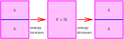
____________________________
The significance of this error is illustrated in figure 24.1. Imagine a container of gas of a certain type, temperature, and pressure that is divided into two equal parts by a sheet of material. The total entropy of this state is 2S, where S is the entropy calculated separately for each half of the body of gas. This follows because the two halves are completely separate systems.
If the divider is now removed, a calculation of the entropy of the full body of gas yields S′ > 2S according to the Gibbs formula, since the calculated entropy doesn’t scale with the amount of gas. Furthermore, replacing the divider restores the system to the initial state in which the total entropy is 2S. Thus, simply inserting or removing the divider, an operation that transfers no heat and does no work on the system, is able to increase or decrease the entropy of the gas at will according to Gibbs. This is at variance with the second law of thermodynamics and is known not to occur. Its prediction by the formula of Gibbs is called the Gibbs paradox. Gibbs was well aware of the serious nature of this problem but was unable to come up with a satisfying solution.
The resolution of the paradox is simply that the Gibbs formula for the entropy of an ideal gas is incorrect. The correct formula is only obtained when the quantum mechanical version of statistical mechanics is used. The failure of Gibbs to obtain the proper entropy was an early indication that classical mechanics had problems on the atomic scale.
We will now calculate the entropy of a body of ideal gas using quantum statistical mechanics. In order to reduce the difficulty of the calculation, we will take a shortcut and assume that the amount of entropy is proportional to the amount of gas. However, the more rigorous calculation confirms that this actually is true.
The quantum mechanical calculation of the states of a particle in a three-dimensional box forms the basis for our treatment of an ideal gas. Recall that a non-relativistic particle of mass M in a one-dimensional box of width a can only support wavenumbers kl = ±πl∕a where l = 1, 2, 3,… is the quantum number for the particle. Thus, the possible momenta are pl = ±ℏπl∕a and the possible energies are
 | (24.1) |
If the box has three dimensions, is cubical with edges of length a, and has one corner at (x,y,z) = (0, 0, 0), the quantum mechanical wave function for a single particle that satisfies ψ = 0 on all the walls of the box is a three-dimensional standing wave,
 | (24.2) |
where the quantum numbers l,m,n are positive integers. You can verify this by examining ψ for x = 0, x = a, etc.
Equation (24.2) is a solution in which the x, y, and z wavenumbers are respectively kx = ±lπ∕a, ky = ±mπ∕a, and kz = ±nπ∕a. The corresponding components of the kinetic momentum are therefore px = ℏkx, etc. The possible energy values of the particle are
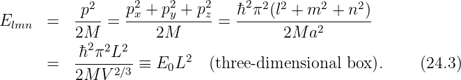
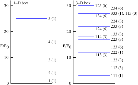
____________________________
Figure 24.2 shows the energy levels of a particle in a one-dimensional and a three-dimensional box. Different values of l, m, and n can result in the same energy in the three-dimensional case. For instance, (l,m,n) = (1, 1, 2), (1, 2, 1), (2, 1, 1) all yield L2 = 6 and hence energy 6E 0. This energy level is thus said to have a degeneracy of 3. Similarly, the states (1, 2, 3), (2, 3, 1), (3, 1, 2), (3, 2, 1), (2, 1, 3), (1, 3, 2) all have the same value of L2, so this level has a degeneracy of 6. However, the state (1, 1, 1) is unique and thus has a degeneracy of 1. From this we see that the degeneracy of an energy level is the number of different physically distinguishable states that have the same energy. Counting the effects of degeneracy, the particle in a three-dimensional box has 60 distinct states for energy less than 30E0, while the one-dimensional box has 5. As E∕E0 increases, this ratio becomes even larger.
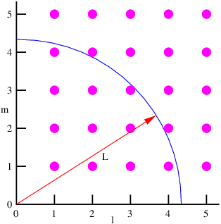
____________________________
In order to compute the entropy of a system, we need to count the number of
states available to the system in a particular band of energies. Figure 24.3 shows
how to count the states with energy less than some limiting value for a particle in
a two-dimensional box. The pie-shaped segment bounded by the arc of radius L
and the l and m axes has an area equal to one fourth the area of a circle of
radius L, or πL2∕4. The dots represent allowed values of the l and m
quantum numbers. One dot, and hence one state, exists per unit area in this
graph, so the above expression tells us how many states exist with
l2 + m2 ≤ L2.
In two dimensions the particle energy is E = (l2 + m2)E 0. Thus, the number of states with energy less than or equal to some maximum energy E is
 | (24.4) |
Similar arguments can be made to calculate the number of states of a particle in a three-dimensional box. The equivalent of figure 24.3 would be a plot with three axes, l, m, and n representing the x, y, and z quantum numbers. The volume of a sphere with radius L is then 4πL3∕3 and the region of the sphere with l,m,n > 0, i. e., an eighth of the sphere, contains real physical states. The result is that
 | (24.5) |
states exist with energy less than E.
An ideal gas of only one molecule isn’t very interesting. Calculating the number of states available to many particles in a box is a bit complex. However, by analogy with the case of multiple harmonic oscillators, we guess that the number of states of an N-particle gas is the number of states available to a single particle to the Nth power multiplied by some as yet unknown function of N, F(N):
 | (24.6) |
(Note that the (π∕6)N from equation (24.5) has been absorbed into F(N).) Substituting E0 = ℏ2π2∕(2MV 2∕3) results in
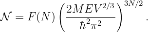 | (24.7) |
Now, π2ℏ2∕(2M) has the units of energy multiplied by volume to the two-thirds power, so we write this combination of constants in terms of constant reference values of E and V :
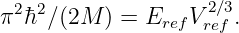 | (24.8) |
Given the above assumption, we can rewrite the number of states with energy less than E as
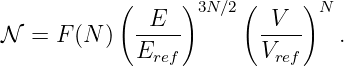 | (24.9) |
We now argue that the combination F(N) must take the form KN-5N∕2 where K is a dimensionless constant independent of N. Substituting this assumption into equation (24.9) results in
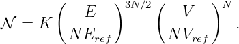 | (24.10) |
It turns out that we will not need the actual values of any of the three constants K, Eref, or V ref.
The effect of the above hypothesis is that the energy and volume occur only in
the combinations E∕(NEref) and V∕(NV ref). First of all, these combinations are
dimensionless, which is important because they will become the arguments of
logarithms. Second, because of the N in the denominator in both cases, they are
in the form of energy per particle and volume per particle. If the energy per
particle and the volume per particle stay fixed, then the only dependence of on
N is via the exponents 3N∕2 and N in the above equation. Why is this
important? Read on!
Recall now that we need to compute the number of states in some small energy interval ΔE in order to get the entropy. Proceeding as for the case of a collection of harmonic oscillators, we find that
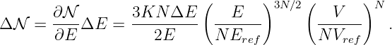 | (24.11) |
The entropy is therefore
![[ ( ) ( ) ]
3- ---E--- --V---
S = kB ln (ΔN ) = N kB 2 ln N E + ln N V (ideal gas),
ref ref](book2221x.png) | (24.12) |
where we have dropped the term kB ln[3KNΔE∕(2E)]. Since this term is not multiplied by the number of particles N, it is unimportant for systems made up of lots of particles.
Notice that this equation has a very important property, namely, that the entropy is proportional to the number of particles for fixed E∕N and V∕N. It thus satisfies the criterion that Gibbs was unable to satisfy in his computation of the entropy of an ideal gas. However, we cannot claim that our calculation is superior to his, because we cheated! The reason we assumed that F(N) = KN-5N∕2 is precisely so that we would obtain this result.
The temperature is the inverse of the E-derivative of entropy:
 | (24.13) |
How does the entropy of a particle in a box change if the volume of the box is changed? The answer to this question depends on how rapidly the volume change takes place. If an expansion or compression takes place slowly enough and no heat is added or removed, the quantum numbers of the particle don’t change.
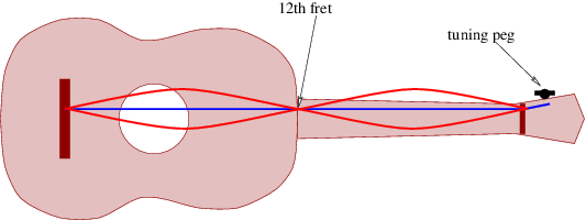
____________________________
This fact may be demonstrated by the tuning of a guitar. A guitar string is tuned in frequency by adjusting the tension on the string with the tuning peg. If the first harmonic mode (corresponding to quantum number n = 2 for particle in a one-dimensional box) is excited on a guitar string as illustrated in figure 24.4, changing the tension changes the frequency of the vibration but it does not change the mode of vibration of the string — for instance, if the first harmonic is initially excited, it remains the primary mode of oscillation.
Slowly changing the volume of a gas consisting of many particles, each with its
own set of quantum numbers, results in the same behavior — changing the
dimensions of the box results in no switching of quantum numbers beyond that
which would normally take place as a result of particle collisions. As a
consequence, the number of states available to the system, Δ, and hence the
entropy, doesn’t change either.
A process that changes the macroscopic condition of a system but that doesn’t change the entropy is called isentropic or reversible adiabatic. The word “isentropic” means at constant entropy, while “adiabatic” means that no heat flows in or out of the system.
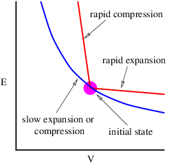
____________________________
If the entropy doesn’t change as a result of a change in volume, then E3∕2V = const according to equation (24.12). Thus, the energy of the gas increases when the volume is decreased and vice versa. This behavior is illustrated in figure 24.5. The change in energy in both cases is a consequence of work done by the gas on the walls of the container as it changes volume — positive in expansion, meaning that the gas loses energy; and negative in compression, meaning that the gas gains energy. This type of energy transfer is the means by which internal energy is converted to useful work.
A rapid expansion of the box has a completely different effect. If the expansion is so rapid that the quantum mechanical waves trapped in the box undergo negligible evolution during the expansion, then the internal energy of the particles in the box does not change. As a consequence, the particle quantum numbers must change to compensate for the change in volume. Equation (24.12) tells us that if the volume increases and the internal energy doesn’t change, the entropy must increase.
A rapid compression has the opposite effect — it does extra work on the material in the box, thus adding internal energy to the gas at a rate in excess of the reversible adiabatic rate. The entropy increases in this type of process as well. Both of these effects are illustrated in figure 24.5.
The pressure p of a gas is the normal force per unit area exerted by the gas on the walls of the chamber containing the gas. If a chamber wall is movable, the pressure force can do positive or negative work on the wall if it moves out or in. This is the mechanism by which internal energy is converted to useful work. We can determine the pressure of a gas from the entropy formula.
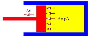
____________________________
Consider the behavior of a gas contained in a cylinder with a movable piston as shown in figure 24.6. The net force F exerted by gas molecules bouncing off of the piston results in work ΔW = FΔx being done by the gas if the piston moves (slowly) out a distance Δx. The pressure is related to F and the area A of the piston by p = F∕A. Furthermore, the change in volume of the cylinder is ΔV = AΔx.
If the gas does work ΔW on the piston, its internal energy changes by
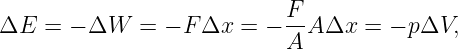 | (24.14) |
assuming that ΔQ = 0, i. e., no heat is added or removed during the change in volume. Solving this for p results in
 | (24.15) |
In the previous section we showed that as long as the change in volume is slow and ΔQ = 0, the entropy does not change. Thus, in the evaluation of ∂E∕∂V , the entropy is held constant.
We can determine the pressure for an ideal gas by solving equation (24.12) for E and taking the V derivative. As we showed in the previous section, E3∕2V is constant for constant entropy processes, which means that
 | (24.16) |
The pressure is then computed to be
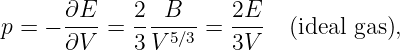 | (24.17) |
where B is eliminated in the last step using equation (24.16). Employing equation (24.13) to eliminate the energy in favor of the temperature, this can be written
 | (24.18) |
which relates the pressure, volume, temperature, and particle number of an ideal gas.
This equation is called the ideal gas law and jointly represents the observed relationships between pressure and volume at constant temperature (Boyle’s law) and pressure and temperature at constant volume (law of Charles and Gay-Lussac). The fact that we can derive it from statistical mechanics is evidence in favor of our quantum mechanical model of a gas.
The formulas for the entropy of an ideal gas (24.12), its temperature (24.13), and the ideal gas law (24.18) summarize our knowledge about ideal gases. Actually, the entropy and temperature laws only apply to a particular type of ideal gas in which the molecules consist of single atoms. This is called a monatomic ideal gas, examples of which are helium, argon, and neon. The molecules of most gases consist of two or more atoms. These molecules have rotational degrees of freedom that can store energy. The calculation of the entropy of such gases needs to take these factors into account. The most common case is one in which the molecules are diatomic, i. e., they consist of two atoms each. In this case simply replacing factors of 3∕2 by 5∕2 in equations (24.12), (24.13), (24.16), and (24.17) results in equations that apply to diatomic gases at ordinary temperatures.
As previously noted, the specific heat of any substance is the amount of heating required per unit mass to raise the temperature of the substance by one degree. For a gas one must clarify whether the volume or the pressure is held constant as the temperature increases — the specific heat differs between these two cases because in the latter situation the added energy from the heating is split between the production of internal energy and the production of work as the gas expands.
At constant volume all heating goes into increasing the internal energy, so ΔQ = ΔE from the first law of thermodynamics. From equation (24.13) we find that ΔE = (3∕2)NkBΔT. If the molecules making up the gas have mass M, then the mass of the gas is NM. Thus, the specific heat at constant volume of an ideal gas is
 | (24.19) |
As noted above, when heat is added to a gas in such a way that the pressure is kept constant as a result of allowing the gas to expand, the added heat ΔQ is split between the increase in internal energy ΔE and the work done by the gas in the expansion ΔW = pΔV such that ΔQ = ΔE + pΔV . In a constant pressure process the ideal gas law (24.18) predicts that pΔV = NkBΔT. Using this and the previous equation for ΔE results in the specific heat of an ideal gas at constant pressure:
 | (24.20) |
Heat engines typically operate by heating and cooling a volume of gas and by compressing or expanding the gas. If these operations are done in a particular order, internal energy can be converted to useful work. We therefore seek to understand how an ideal gas reacts to the addition and subtraction of internal energy and to the change in the volume of the gas.
The equation for the entropy of an ideal gas and the ideal gas law contain the information we need. The entropy of an ideal gas is a function of its internal energy E and its volume V . (We assume that the number of molecules in the gas remains fixed.) Thus, a small change ΔS in the entropy can be related to small changes in the energy and volume as follows:
 | (24.21) |
We know that ∂S∕∂E = 1∕T. Using equation (24.12) we can similarly calculate ∂S∕∂V = NkB∕V = p∕T, where the ideal gas law is used in the last step to eliminate NkB in favor of p. Substituting these into the above equation, multiplying by T, and solving for pΔV results in
 | (24.22) |
where we have recognized pΔV = ΔW to be the work done by the gas on the piston.
We are now in a position to investigate the conversion of internal energy to useful work. If the gas is allowed to push the piston out in a reversible adiabatic manner, then ΔS = 0 and energy is converted with 100% efficiency from internal form to work. This work could in principle be used to run an electric generator, stretch springs, power an automobile, etc.
Unfortunately, a piston in a cylinder that can only extract energy during a single expansion wouldn’t be very useful — it would be like an automobile engine that only worked for half a turn of the crankshaft and then had to be replaced! If the piston is simply pushed back into the cylinder, then the macroscopic energy gained from the initial expansion would be converted back into internal energy of the gas, resulting in zero net creation of useful work.
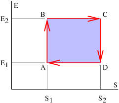
____________________________
The trick to obtaining non-zero useful work from the expansion and contraction of a gas is to add heat to the gas before the expansion and extract heat from it before the recompression. This makes the gas cooler in the compression than in the expansion. The pressure is therefore less in the compression and the work needed to compress the gas is less than that produced in the expansion.
Figure 24.7 shows a particular way of executing a complete cycle of expansion and compression of the gas that results in a net conversion of internal energy to useful work. Assuming that the gas has initial entropy and internal energy S1 and E1 at point A in figure 24.7, the gas is first compressed in reversible adiabatic fashion to point B. The entropy doesn’t change in this compression but the internal energy increases from E1 to E2. The work done by the gas is negative and equals WAB = E1 - E2.
The gas then is allowed to slowly expand (so that the expansion is reversible), moving from point B to point C in figure 24.7 in such a way that its internal energy doesn’t change. From equation (24.22) we see that WBC = T2(S2 -S1) for this segment of the expansion. However, heat must be added to the gas equal in amount to the work done in order to keep the internal energy fixed: Q2 = T2(S2 - S1).
From point C to point D the gas expands further but in this segment the expansion is reversible adiabatic so that the entropy change is again zero. Thus, WCD = E2 - E1.
Finally, the gas is slowly compressed from point D to point A in a constant internal energy process. Keeping the internal energy fixed means that the (negative) work done by the gas in this segment is WDA = T1(S1 - S2). Furthermore, heat equal to the work done on the gas by the piston must be removed from the gas in order to keep the internal energy constant: Q1 = -WDA = T1(S2 - S1). The net work done by the gas over the full cycle is obtained by adding up the contributions from each segment:
The energy source for this work is internal energy at temperature T2. As demanded by energy conservation, W = Q2 - Q1. The fraction of the internal energy Q2 that is converted to useful work in this cycle is
 | (24.24) |
This quantity ϵ is called the thermodynamic efficiency of the heat engine. Notice that it depends only on the ratio of the lower and upper temperatures, expressed in absolute or Kelvin form. The smaller this ratio, the larger the thermodynamic efficiency.
Heat engines normally work via repeated cycling around some loop such as described above. The particular cycle we have discussed is called the Carnot cycle after the 19th century French scientist Sadi Carnot. Heat is accepted from a high temperature heat source, created, for example, by burning coal in a power plant. Excess heat is disposed of in the atmosphere or in some source of running water such as a river. Notice that the ability to get rid of excess heat at low temperature is as important to a heat engine as the supply of heat at a high temperature.
Many cycles for converting heat to work are possible — these are represented by different closed trajectories in the S-E plane. However, the Carnot cycle is special for two reasons: First, all heat absorbed by the system is absorbed at a single temperature T2, and all heat rejected from the system is rejected at a single temperature T1. This allows the expression of the efficiency simply in terms of the two temperatures. Second, the Carnot cycle is reversible, which means that no net entropy is generated.
A Carnot engine running backwards acts as a refrigerator. Heat ΔQ1 is extracted at temperature T1 from the box being cooled with the aid of externally supplied work W. An amount of heat Q2 = W + Q1 is then transferred to the environment at temperature T2 > T1. Equation (24.24) gives the ratio of W to Q2 in this case, as well as when the heat engine is run in the forward direction. This may be verified by tracing the cycle in figure 24.7 in reverse.
In analyzing heat engines and refrigerators it is generally easier to go back to basic principles than it is to use equations such as (24.23) and (24.24). In particular, for a Carnot engine in which heat Q2 is being extracted from the high temperature reservoir (T2) and heat Q1 is being added to the low temperature reservoir (T1), conservation of energy says that the useful work extracted is W = Q2 - Q1, and that the total combined entropy change in the warm and cold reservoirs is ΔS = -Q2∕T2 + Q1∕T1 = 0. (Note that the reservoir providing energy has a minus sign, while the reservoir accepting energy has a plus sign.) Given these two relationships, any two of Q1, Q2, and W can be determined if the third is known. For a refrigerator, the higher temperature reservoir accepts energy while the lower temperature reservoir (generally the interior of the refrigerator) and the work term provide energy. This changes the signs of all three energy flows. If the machine is not a perfectly efficient Carnot engine, then ΔS > 0 whether the machine is a heat engine or a refrigerator, and one deals with inequalities rather than equalities.
Perpetual motion machines are devices that are purported to create useful work for “nothing” by violating some physical principle. Generally they are divided into two types, perpetual motion machines of the first and second kinds. Perpetual motion machines of the first kind violate the conservation of energy, while perpetual motion machines of the second kind violate the second law of thermodynamics. It is the latter type that we address here.
We commonly hear talk of an “energy crisis”. However, it is clear to all physicists that such a crisis, if it exists, is actually an “entropy crisis”. Energy beyond the most extravagant projected needs of mankind exists in the form of internal energy of the earth. Furthermore, one cannot possibly “waste” energy, because energy can neither be created nor destroyed.
The real problem is that internal energy can only be tapped if two reservoirs of internal energy exist, one at high temperature and one at low temperature. Heat engines depend on this temperature difference to operate and if all internal energy exists at the same temperature, no conversion of internal energy to useful work is possible, at least using the Carnot cycle.
One naturally inquires as to whether some cycle exists that is more efficient than the Carnot cycle. In other words, does there exist a heat engine operating between temperatures T2 and T1 that extracts more work from the high temperature heat input Q2 than ϵQ2? Recall that ϵ = 1 - T1∕T2 is the thermodynamic efficiency of the Carnot engine.
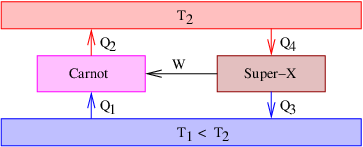
____________________________
Let’s suppose that an inventor has presented us with the “Super-X machine”, which is purported to have a thermodynamic efficiency greater than a Carnot engine. Figure 24.8 shows how we could set up an experiment in our laboratory to test the inventor’s claim. The Carnot engine runs in reverse as a refrigerator, emitting heat Q2 to the upper reservoir, absorbing Q1 from the lower reservoir, and using the work W = Q2 -Q1 = ϵQ2 from the Super-X machine. The Super-X machine is operated in heat engine mode, emitting Q3 to the lower reservoir and absorbing Q4 = Q3 + W < W∕ϵ from the upper reservoir. The inequality indicates that the ratio of work produced and heat extracted from the upper reservoir, W∕Q4, is greater for the Super-X machine than for an equivalent Carnot engine.
Let us examine the net heat flow out of the upper reservoir, Qupper = Q4 -Q2. Since Q4 < W∕ϵ = Q2, we find that Qupper < 0. In other words, the Super-X machine is extracting less heat from the upper reservoir than the Carnot engine is returning to this reservoir using the work produced by the Super-X machine. The source of this energy is the lower reservoir, from which an equivalent amount of heat is being extracted. The net effect of these two machines working together is a spontaneous transfer of heat from a lower to a higher temperature, since no outside energy source or entropy sink is needed to make it operate. This is a violation of the second law of thermodynamics. Therefore, the Super-X machine, if it truly works, is a perpetual motion machine of the second kind.
Though there have been many claims, no perpetual motion machine has been convincingly demonstrated. Thus, heat engines are apparently incapable of converting all of the internal energy supplied to them to useful work, as this would require either an infinite input temperature or a zero output temperature. As we have demonstrated, this source of inefficiency is intrinsic to all heat engines and is in addition to the usual sources of inefficiency such as friction and heat loss from imperfect insulation. No heat engine, no matter how perfectly designed, can overcome this intrinsic inefficiency.
As a result of the second law of thermodynamics, we see that real heat engines, which are always less efficient than Carnot engines, produce useful work, W,
 | (24.25) |
where Q2 is the amount of heat energy extracted from the upper reservoir. On the other hand, refrigerators transfer heat Q2 to the upper reservoir in the amount
 | (24.26) |
where W is the work done on the refrigerator.
for N particles. Eliminate a in favor of the box area A.
These calculations are relevant to atoms that can move freely around on a surface, but cannot escape it for energetic reasons.
This appendix contains various useful constants and conversion factors as well as information on the International System of Units.
“SI” is the French abbreviation for the International System of Units, the system used universally in science. See http://physics.nist.gov/cuu/Units/ for the last word on this subject. This treatment is derived from the National Institute of Science and Technology (NIST) website.
The most fundamental units of measure are length (meters; m), mass (kilograms; kg), time (seconds; s), electric current (ampere; A), temperature (kelvin; K), amount of a substance (mole; mol), and the luminous intensity (candela; cd). The candela is a rather specialized unit related to the perceived brightness of a light source by a “standard” human eye. As such, it is rather anthropocentric and hardly seems to merit the designation “fundamental”. The mole is also less fundamental than the other units, as it is simply a convenient way to refer to a multiple of Avogadro’s number of atoms or molecules.
Fundamental units can be combined to form derived units with special names. Some of these derived units are listed below.
Fundamental and derived SI units can have multipliers expressed as prefixes, e. g., 1 km = 1000 m. The NIST website points out a minor irregularity with the fundamental unit of mass, the kilogram. This already has the multiplier “kilo” prefixed to the unit “gram”. In this case 1000 kg is written 1 Mg, not 1 kkg, etc. SI multipliers are listed below as well.
| Name | Abbrev. | Units | Meaning |
| hertz | Hz | s-1 | frequency (cycles/sec) |
| (unnamed) | s-1 | angular frequency (radians/sec) | |
| newton | N | kg m s-2 | force |
| pascal | Pa | N m-2 | pressure |
| joule | J | N m | energy |
| watt | W | J s-1 | power |
| coulomb | C | A s | electric charge |
| volt | V | N m C-1 | scalar potential |
| (unnamed) | N s C-1 | vector potential | |
| (unnamed) | V m-1 | electric field | |
| tesla | T | N s C-1 m-1 | magnetic field |
| (unnamed) | V m | electric flux | |
| weber | Wb | T m2 | magnetic flux |
| volt | V | V | electric circulation (EMF) |
| (unnamed) | T m | magnetic circulation | |
| farad | F | C V-1 | capacitance |
| ohm | Ω | V A-1 | resistance |
| henry | H | V s2 C-1 | inductance |
| Multiplier | Name | Prefix |
| 1024 | yotta | Y |
| 1021 | zetta | Z |
| 1018 | exa | E |
| 1015 | peta | P |
| 1012 | tera | T |
| 109 | giga | G |
| 106 | mega | M |
| 103 | kilo | k |
| 102 | hecto | h |
| 101 | deka | da |
| 10-1 | deci | d |
| 10-2 | centi | c |
| 10-3 | milli | m |
| 10-6 | micro | μ |
| 10-9 | nano | n |
| 10-12 | pico | p |
| 10-15 | femto | f |
| 10-18 | atto | a |
| 10-21 | zepto | z |
| 10-24 | yocto | y |
An older system of scientific units is the CGS system. This system is still used widely in certain areas of physics. The fundamental units of length, mass, and time are as implied by the title given above. The most common CGS derived units are those for force (1 dyne = 10-5 N) and energy (1 erg = 10-7 J).
Electromagnetism is expressed in several different ways in CGS units. Electromagnetic quantities in CGS not only have different units than in SI, they also have different physical dimensions, with different versions differing among themselves. The most common variant of CGS electromagnetic units is called “Gaussian” units. This variant is advocated by some physicists, though many others consider the whole subject of CGS electromagnetic units to be a terrible mess! SI units for electromagnetism are used in this text and CGS units will not be discussed further here.
| 1 lb = 4.448 N |
| 1 ft = 0.3048 m |
| 1 mph = 0.4470 m s-1 |
| 1 eV = 1.60 × 10⁻¹⁹ J |
| 1 mol = 6.022 × 10²³ molecules |
| (One mole of carbon-12 atoms has a mass of 12 g.) |
| 1 gauss = 10-4 T (CGS unit of magnetic field) |
| 1 millibar = 1 mb = 100 Pa (Old unit of pressure) |
When faced with solving an algebraic equation to obtain a numerical answer, solve the equation symbolically first and then substitute numbers. For example, given the equation
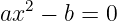 | (A.1) |
where a = 2 and b = 8, first solve for x,
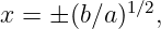 | (A.2) |
and then substitute the numerical values:
 | (A.3) |
This procedure is far better than substituting numbers first,
 | (A.4) |
and then solving for x. Solving first and then substituting has two advantages: (1) It is easier to make algebraic manipulations with symbols than it is with numbers. (2) If you decide later that numerical values should be different, then the entire solution procedure doesn’t have to be repeated, only the substitutions at the end.
In numerical calculations, keep only one additional digit beyond those present in the least accurate input number. For instance, if you are taking the square root of 3.4, your calculator might tell you that the answer is 1.843908891. The answer you write down should be 1.84. Keeping all ten digits of the calculator’s answer gives a false sense of the accuracy of the result.
Round the result up if the digit following the last significant digit is 5 or greater and round it down if it is less than 5. Thus, the square root of 4.1, which the calculator tells us is 2.049390153, should be represented as 2.05 rather than 2.04.
It is easy to make mistakes when changing the units of a quantity. Adopting a systematic approach to changing units greatly reduces the chance of error. We illustrate a systematic approach to this problem with an example in which we change the units of acceleration from meters per second squared to kilometers per minute squared:
| Symbol | Value | Meaning |
| h | 6.63 × 10⁻³⁴ J s | Planck’s constant |
| ℏ | 1.06 × 10⁻³⁴ J s | h∕(2π) |
| c | 2.998 × 10⁸ m s-1 | speed of light |
| G | 6.67 × 10⁻¹¹ m3 s-2 kg-1 | universal gravitational constant |
| kB | 1.38 × 10⁻²³ J K-1 | Boltzmann’s constant |
| σ | 5.67 × 10⁻⁸ W m-2 K-4 | Stefan-Boltzmann constant |
| K | 3.67 × 10¹¹ s-1 K-1 | thermal frequency constant |
| ϵ0 | 8.85 × 10⁻¹² C2 N-1 m-2 | permittivity of free space |
| μ0 | 4π × 10-7 N s2 C-2 | permeability of free space (= 1∕(ϵ 0c2)). |
| Symbol | Value | Meaning |
| e | 1.60 × 10⁻¹⁹ C | fundamental unit of charge |
| me | 9.11 × 10⁻³¹ kg = 0.511 MeV | mass of electron |
| mp | 1.672648 × 10⁻²⁷ kg = 938.280 MeV | mass of proton |
| mn | 1.674954 × 10⁻²⁷ kg = 939.573 MeV | mass of neutron |
| Symbol | Value | Meaning |
| Me | 5.98 × 1024 kg | mass of earth |
| Mm | 7.36 × 10²² kg | mass of moon |
| Ms | 1.99 × 1030 kg | mass of sun |
| Re | 6.37 × 10⁶ m | radius of earth |
| Rm | 1.74 × 10⁶ m | radius of moon |
| Rs | 6.96 × 10⁸ m | radius of sun |
| Dm | 3.82 × 10⁸ m | earth-moon distance |
| Ds | 1.50 × 10¹¹ m | earth-sun distance |
| g | 9.81 m s-2 | earth’s surface gravity |
Absorption lines, 122
Aharonov-Bohm effect, 18, 20
Alpha particle, 96
Ampère’s law, 75, 80, 81
Maxwell’s term, 81
Ampère, André-Marie, 80
Angular momentum, 1, 112
conservation of, 9
orbital, 112
quantum mechanics, 112
spin, 112
Antiparticles, 16, 96, 128
and four-momentum, 30
and negative energies, 29
annihilation, 29
backward in time, 29
pair creation/destruction, 113
pair production, 29
Atom, 94, 112
Rutherford model, 96
Atomic mass number (A), 96, 145
Atomic nucleus, 94, 96, 142
analogy with molecules, 142
and chemistry, 147
measurement of size, 104
Atomic number (Z), 96, 145
Atomic spectra, 120
spectral lines, 121
Baryon, 127
definition, 127
number, 128
Becquerel, Henri, 96
Binding energy, 12
between quarks, 133
maximum per nucleon, 147
of alpha particle, 149
of atomic nucleus, 143, 145
of hydrogen atom, 117
per nucleon, 145
Bjorken, James, 105
Black body radiation, 164
Bohr magneton, 116
Bohr radius, 118
Bohr, Niels, 118
Boltzmann, Ludwig, 177
Bose-Einstein condensate, 115
Boson, 113
Boyle’s law, 197
Brahe, Tycho, 9
Capacitance, 76
Capacitor, 75
definition, 75
parallel plate, 75
Carnot cycle, 199
(no) entropy generated, 201
refrigerator, 201
temperature reservoirs, 201
thermodynamic efficiency, 202
Carnot, Sadi, 200
Chadwick, James, 96
Charge to mass ratio, 95
electrons, 95
Millikan experiment, 95
positive ions, 95
Charged particle motion, 38, 50
conservative electric field, 38
constant electric field, 38
constant magnetic field, 40
crossed electric and magnetic fields, 42
Chemical element, 147
Circulation of vector field, 75, 78
Conductor, 43
Cosmic rays, 101
Coulomb’s law, 56, 57, 81
and relativity, 61
Cowan, Clyde, 97
Crookes tube, 94
Curie temperature, 116
Curie, Marie, 96
Curie, Pierre, 96
Cyclotron frequency, 41
Deep inelastic scattering, 104
and structure of proton, 104
Diamagnetism, 116
Diffraction, 94
and wavelength, 98
de Broglie relationship, 99
of moonlight, 97
opening angle, 98
Displacement current, 81
Einstein, Albert, 23
Elastic collision, 102
Electric battery, 86
Electric charge, 36–41, 58
conservation of, 70
in conductor, 43
in insulators, 44
in parallel plate capacitor, 76
line of, 59, 63
point, 56
potential energy, 40
sheet of, 59
Electric circuit, 75, 89
Electric current, 43
charge carrier, 44
definition, 43
magnetic force, 44
Electric dipole, 39
dipole moment, 39
electric force, 39
electric torque, 39
potential energy, 40
tendency to align with field, 40
Electric field, 37, 38, 40, 46
conservative, 38, 46
energy, 75, 85
energy density, 87
from line of charge, 59
from sheet of charge, 65
in parallel plate capacitor, 76
in plane wave, 68
non-conservative, 38, 46
Electric flux, 57, 59
Electric generator, 36, 49, 50, 79, 86
principle of operation, 49
Electric motor, 36, 46
principle of operation, 46
Electromagnetic fields, 36
dependence on reference frame, 42
generation by charge, 56
Electromagnetic forces, 36–38, 40, 41, 44, 45, 47
Electromagnetic radiation, 66
dispersion relation, 81
from accelerated charge, 67
from particle collisions, 67
Electromagnetism, 16, 23, 36
as a gauge theory, 16
Electromotive force (EMF), 47
Electron, 94
discovery of, 95
Electroweak theory, 133
and CP non-conservation, 136
and electromagetism, 135
and parity non-conservation, 136
and quark flavor, 136
and weak force, 135
intermediary particles, 135
mass of W and Z particles, 135, 136
range of force, 137
weak coupling constant, 136
EMF, 47, 86
and scalar potential, 49
electric circulation, 79
Energy, 1, 16
kinetic, 16
relation to velocity, 18
macroscopic, 159
microscopic or internal, 159
potential, 17
relation to force, 17, 20
rest energy, 24
rest, 16, 118
total, 16, 19
relation to frequency, 18
Entropy, 177
and number of available states, 178
definition, 177
of ideal gas, 193
of two systems combined, 180
Escape velocity, 11
Faraday’s law, 49, 79, 81, 84
Faraday, Michael, 38
Fermion, 113
Ferromagnetism, 116
Feynman, Richard, 16, 29, 105
Fine structure constant, 118
First law of thermodynamics, 161
Four-momentum, 16, 17
conservation of, 25
potential, 18, 36
Four-potential, 36, 42, 61, 62, 81
for moving charge, 62
for plane wave, 68
Frictional force, 164
in fluids, 166
kinetic friction, 165
static friction, 165
Fundamental forces, 97
electromagnetic, 97, 127
gravity, 97
strong, 97, 105, 127, 129
weak, 97, 127, 133
Gamma ray, 148
Gauge invariance, 37
Gauge theory, 16, 23, 28, 36
electromagnetism, 16
strong interactions, 24
weak interactions, 24
Gauss’s law for electric field, 56, 57, 59, 76, 81
Gauss’s law for gravity, 5
multiple masses, 6
Gauss’s law for magnetic field, 56, 61, 81
Geiger, Hans, 96, 99
Geiger-Marsden experiment, 94, 96, 99, 103
and size of nucleus, 100
Gibbs paradox, 188
Gibbs, J. Willard, 170, 187
Glashow, Sheldon, 135
Gluon, 105, 129
and strong force, 129
color combinations, 132
Grand unification, 137
Gravitational field, 2
addition of fields, 2
curvature of spacetime, 24
dimensions, 2
sphere of mass, 6
Gravitational flux, 3, 57
and gravitational field, 4
direction, 4
water flow analogy, 4
Graviton, 128
and gravitational force, 128
Gravity
a central force, 9
conservation of energy and angular momentum, 10
conservative force, 10
general relativity, 24
Gravity and relativity
geodesic curve, 8
gravitational waves, 8
relativity, 7
Gyromagnetic ratio, 115
of electron, 115
Hadron, 127
definition, 127
made of quarks, 129
Heat, 156
as energy transfer, 159
conduction, 156
is a verb, 161
Heat conduction, 161
law of, 161
Heat engine, 161, 186, 198
Henry, Joseph, 38
Higgs field, 24
Higgs particle, 135
Higgs, Peter, 24
Hofstadter, Robert, 103
Hydrogen atom, 117
Balmer series, 121
energy levels, 118
degenerate, 119
ground state energy, 117
Lyman series, 121
orbital z component quantum number, 119
orbital angular momentum quantum number, 119
Paschen series, 122
principal quantum number, 118
spin orientation quantum number, 119
Ideal gas, 186
constant entropy process, 196
constant internal energy process, 194
definition, 186
diatomic, 197
entropy, 187
monatomic, 197
slow and fast expansions, 193
specfic heat at constant pressure, 198
specific heat at constant volume, 197
Ideal gas law, 197
Inductor, 82
parallel plate, 82
Inelastic collision, 102
Insulator, 43
Intermediary particle, 16, 28
fundamental, 128
postulated by Yukawa, 101
Isotopes, 147
of hydrogen, 147
of very heavy elements, 149
Kaon, 128
Kepler’s first law, 9
Kepler’s second law, 9
and angular momentum, 9
Kepler’s third law, 9
circular orbits, 10
Kepler, Johannes, 9
Kinetic energy, 11, 12
Kirchhoff’s laws, 75, 88
approximations, 89
Lambda particle, 128
Laser, 122
Law of Charles and Gay-Lussac, 197
Law of gravitation, 1
electric equivalent, 57
gravitational constant, 1
Lenz’s law, 84
Lepton, 127
as fundamental particle, 129
definition, 127
number, 128
Line of stability, 147
Lorentz contraction, 64
Lorentz force, 37, 41
Lorenz condition, 23, 37, 68, 78, 81
origin, 69
time-dependent scalar potential, 81
Magnetic circulation, 80
around a current, 80
in a capacitor, 80
Magnetic dipole, 44
current loop, 45
dipole moment, 45, 115
direction of, 45
potential energy, 45
Magnetic field, 37, 38
changing with time, 38
energy, 75, 85
energy density, 87
from changing electric field, 47
from moving charge, 61
from moving line of charge, 63, 64
from moving sheet of charge, 66, 83
in a capacitor, 77
in plane wave, 68
lines, 63
Magnetic flux, 48, 61
Magnetic inductance, 84
Magnetic induction, 75, 82
Magnetic monopole, 61
Marsden, Ernest, 96, 99
Matter wave, 20
refraction of, 20
Maxwell’s equations, 81
Maxwell, James Clerk, 80
Meson, 128
definition, 128
Millikan, Robert, 95
Momentum, 16
canonical, 18
kinetic, 18, 19
relation to velocity, 18
potential, 17–19, 23
relation to force, 20
time-varying, 22
total, 18
relation to wave vector, 18
Momentum:transfer in collisions, 28
Muon, 101
decay, 102
discovery in cosmic rays, 101
Neutrino, 97
discovery, 97
electron neutrino, 102
in beta decay, 97
mu neutrino, 101
Neutron, 96
decay, 97, 136
discovery of, 96
number in nucleus (N), 96
Newton’s second law, 21, 38
Newton, Isaac, 1, 9
Nuclear fission, 152
by capture of slow neutron, 153
spontaneous, 154
Nuclear force, 144
Nuclear fusion, 151
in supernovae, 152
Nucleon, 96, 142
Ohm’s law, 75, 84
Orbits, 9
aphelion, 12
elliptical orbit, 12
hyperbolic orbit, 12
impact parameter, 12
maximum angular momentum, 13
parabolic orbit, 12
perihelion, 12
Paramagnetism, 116
Particle accelerators, 94, 102
Particle in three-dimensional box, 188
Particle mass, 95
electron, 95
positive ions, 95
Parton, 105
Pauli exclusion principle, 114, 144
Pauli, Wolfgang, 97
Permeability of free space, 64
Permittivity of free space, 56
Perpetual motion machine, 201
of the first kind, 201
of the second kind, 201
and second law of thermodynamics, 201
Photon, 36, 66, 96
and electromagnetic force, 128
Pion, 101, 128
decay, 101
discovery in cosmic rays, 101
Plane wave, 68
Positron, 96
Potential energy, 12, 16, 17, 36, 38, 40, 45, 46
gravitational, 10
of electric charges, 56
Potential momentum, 17, 36
Pressure, 195
Proper time, 27
Proton, 96
parton model, 108
Quantum chromodynamics, 132
color charge, 132
color quantum number, 132
coupling constant, 133
Quantum mechanical states, 170
multiple particles in box, 191
number of, 170
of a brick, 170, 172
of harmonic oscillator, 172
of particle in 3-D box, 190
Quantum mechanics, 16, 112
identical particles, 113
of gravity, 139
of two particles, 113
relativistic, 16
Quark, 97, 105
as fundamental particle, 129
baryon number, 131
charge on, 129
color, 132
confinement, 132
flavor, 129
strong force, 129
Rabi, I. I., 102
Radioactive decay, 96, 148
alpha decay, 96, 149
beta decay, 96, 148, 149
discovery of, 96
gamma decay, 96, 148
half-life, 151
law of, 150
Range of interaction, 28
intermediary particle mass, 28
Reines, Frederick, 97
Relativity, 16
and magnetism, 56
force, 17
force at a distance, 16, 25
negative energies, 16
negative energy, 136
potential energy, 16
principle of, 17, 23
Resistence, 84
Resistivity, 85
Resistor, 75, 85
Rest energy of nucleus, 149
Rutherford, Ernest, 96, 99
Salam, Abdus, 135
Scalar potential, 36, 37, 59, 62
and EMF, 49
and potential energy, 36
from charge, 56
from line of charge, 63
from sheet of charge, 65
in parallel plate capacitor, 76
Scattering, 94
Second law of thermodynamics, 178, 183, 186
and irreversible entropy generation, 183
and temperature equilibration, 183
Snell’s law, 21
Spacetime Pythagorean theorem, 62
Specific heat, 160
of a brick, 182
Spectroscope, 121
Standard model, 127
color charge, 142
electroweak theory, 133
particle generations, 137
strong interaction, 129, 143
Statistical mechanics, 170
classical, 187
quantum, 188
Stefan’s law, 163
Stern-Gerlach experiment, 124
Stimulated emission, 122
Stirling approximation, 176
Storage rings and colliders, 107
Strange particle, 128
Strangeness, 128
(non)conservation, 128
Superconductivity, 115
Superfluidity, 115
Temperature, 156
Celsius scale, 158
equilibration, 156, 181
Kelvin scale, 158
measurement, 156
of ideal gas, 193
reservoirs, 186
thermodynamic definition, 182
Thermal conductivity, 162
Thermal emissivity, 163
Thermal expansion
coefficient of, 157
Thermal radiation, 157, 162
flux, 163
Thermodynamic efficiency, 200
Thermodynamics, 156
Thomson, J. J., 94
Two-jet events, 108
from electron-positron collisions, 109
from proton-antiproton collisions, 108
Uncertainty principle, 109, 117, 170
Vector potential, 36, 37
and potential momentum, 36
from moving line of charge, 63
from moving sheet of charge, 65, 83
in a capacitor, 78
in an inductor, 82
longitudinal component (in radiation), 68
transverse component (in radiation), 68
Virial theorem, 118
Virtual mass, 67
of electron, 67
of photon, 68
Virtual particle, 16, 26, 27, 133
as an intermediary particle, 28
massive, 28
massless, 28
velocity, 26
Viscosity, 166
in a gas, 167
in a liquid, 167
Voltage drop, 84
Water, properties of, 158
Weinberg, Steven, 135
World line, 27
Yukawa, Hideki, 101